
Welcome back to part three of the series on creating recommendations with the H&M dataset. To recap on the previous posts, here are the links.
- Part 1 - loading the data and EDA
- Part 2 - image based recommendations
This week we’ll be focussing on creating recommendations using a collaborative filtering approach. Outside of the product metadata supplied as part of the H&M dataset, there is no explicit feedback available from the customer about the product i.e. reviews or ratings. Given this, the focus of this post will be on how we can use implicit feedback to create these recommendations.
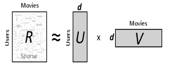
This approach to recommendations is a form of matrix factorization where we decompose the user-item purchase matrix into to a user matrix and an item matrix with a predetermined number of latent factors as in the diagram below.
I’ll defer all the gory details of how this process is done and optimized but here are a couple of good resources if anyone wants to read further:
- Collaborative Filtering for Implicit Feedback Datasets.
- Alternating Least Squares for Implict Datasets.
We’ll be using the Alternating Least Squares algorithm for this approach which is available as part of the Implicit package. I also lean heavily (read blatantly steal) on the code from this excellent blog post by Ethan Rosenthal which I’d advise anyone to check out for a thorough run through of recommendations with implicit feedback.
Getting Started
To start we’ll import some packages and load some file paths…the usual stuff.
# Load packages
from pathlib import Path
from matplotlib import image
import matplotlib.pyplot as plt
import numpy as np
import pandas as pd
import implicit
from scipy import sparse
import datetime as dt
from neo4j import GraphDatabase

# Get all image file names
IMAGE_DIR = '/Users/grantbeasley/Downloads/images/'
images = Path(IMAGE_DIR)
all_files = [image for folder in images.iterdir() if not folder.name == '.DS_Store' for image in folder.iterdir() if image.suffix == '.jpg']

# Load the transaction data
uri = "bolt://localhost:7687"
driver = GraphDatabase.driver(uri, auth=("neo4j", "password"))

with driver.session(database='neo4j') as session:

    query = """
    MATCH (c:Customer)-[pur:PURCHASED]->(p:Product)
    RETURN
      pur.t_date as t_dat, c.id as customer_id, p.code as article_id
    """

    results = session.run(query)

    purchases = [(record['t_dat'], record['customer_id'], record['article_id']) for record in results]

purchases = pd.DataFrame(purchases, columns=['t_dat', 'customer_id', 'article_id'])
Another thing to note is that the most recent purchase in the transactions dataset is ‘2020-09-22’ meaning we’ll be making recommendations for the week proceeding that date.
Transaction Data
A quick overview into the transaction data gives us an insight into the dataset.
n_users = purchases['customer_id'].unique().shape[0]
n_items = purchases['article_id'].unique().shape[0]

print('Number of users: {}'.format(n_users))
print('Number of models: {}'.format(n_items))
print('Sparsity: {:4.3f}%'.format(float(purchases.shape[0]) / float(n_users*n_items) * 100))

>>> Number of users: 1362281
>>> Number of models: 104547
>>> Sparsity: 0.022%
As we can see from the Sparsity value, the data is incredibly sparse which is often the case for user-item type datasets. Quoting Ethan Rosenthal blog post:
While implicit recommendations excel where data is sparse, it can often be helpful to make the interactions matrix a little more dense. We limited our data collection to models that had at least 5 likes. However, it may not be the case that every user has liked at least 5 models. Let’s go ahead and knock out users that liked fewer than 5 models. This could possibly mean that some models end up with fewer than 5 likes once these users are knocked out, so we will have to alternate back and forth knocking users and models out until things stabilize.
And off the back of this, we can borrow the function from the blog post to help decrease the sparsity of the data.
def threshold_likes(df, user_min, article_min):
    n_users = df['customer_id'].unique().shape[0]
    n_items = df['article_id'].unique().shape[0]
    sparsity = float(df.shape[0]) / float(n_users*n_items) * 100
    print('Starting likes info')
    print('Number of users: {}'.format(n_users))
    print('Number of models: {}'.format(n_items))
    print('Sparsity: {:4.3f}%'.format(sparsity))

    done = False
    while not done:
        starting_shape = df.shape[0]
        article_counts = df.groupby('customer_id')['article_id'].count()
        df = df[~df['customer_id'].isin(article_counts[article_counts < article_min].index.tolist())]
        user_counts = df.groupby('article_id')['customer_id'].count()
        df = df[~df['article_id'].isin(user_counts[user_counts < user_min].index.tolist())]
        ending_shape = df.shape[0]
        if starting_shape == ending_shape:
            done = True

    assert(df.groupby('customer_id')['article_id'].count().min() >= article_min)
    assert(df.groupby('article_id')['customer_id'].count().min() >= user_min)

    n_users = df['customer_id'].unique().shape[0]
    n_items = df['article_id'].unique().shape[0]
    sparsity = float(df.shape[0]) / float(n_users*n_items) * 100
    print('Ending likes info')
    print('Number of users: {}'.format(n_users))
    print('Number of models: {}'.format(n_items))
    print('Sparsity: {:4.3f}%'.format(sparsity))
    return df

purchases_dense = threshold_likes(purchases, 5, 5)

>>> Starting likes info
>>> Number of users: 1362281
>>> Number of models: 104547
>>> Sparsity: 0.022%
>>> Ending likes info
>>> Number of users: 925154
>>> Number of models: 91511
>>> Sparsity: 0.036%
As we can see from the output, we lose 437127 users and 13036 items from the dataset by running this function. As always, there’s a trade off between the sparsity of the data and the quality of recommendations. We could maintain more users and items in the DataFrame but the increased sparsity of the data may lead to poorer recommendations and vice versa.
Creating New User and Item ID’s
Now we’ve reduced the size of the dataset, we need to map some new user IDs and item IDs to the remaining users and items which can be used to form the row and columns indices of the sparse matrices we need to create.
# Create mappings
article_to_idx = {}
idx_to_article = {}
for (idx, aid) in enumerate(purchases_dense['article_id'].unique().tolist()):
    article_to_idx[aid] = idx
    idx_to_article[idx] = aid

user_to_idx = {}
idx_to_user = {}
for (idx, uid) in enumerate(purchases_dense['customer_id'].unique().tolist()):
    user_to_idx[uid] = idx
    idx_to_user[idx] = uid
And subsequently create the sparse user-item matrix from the dataframe.
def map_ids(row, mapper):
    return mapper[row]

I = purchases_dense['customer_id'].apply(map_ids, args=[user_to_idx]).values
J = purchases_dense['article_id'].apply(map_ids, args=[article_to_idx]).values
V = np.ones(I.shape[0])
purchases_sparse = sparse.coo_matrix((V, (I, J)), dtype=np.float64)
purchases_sparse = purchases_sparse.tocsr()
There are a few things we need to remember when dealing with implicit feedback:
- No negative feedback - user behaviour allows us to infer what they probably like, however it’s incredibly difficult to infer which products a user doesn’t like - just because a user hasn’t purcahsed an item doesn’t mean they don’t or would not like it. This in unlike a movie feedback where a user could give a poisitive or negative review from which we could derive whether a user likes or doesn’t like it.
- Implicit feedback is noisy - passively tracking user behaviour only allows us to guess their preferences. A user may purchase a product but actually not like it for example.
- Explicit feedback indicates preference, implicit feedback indicates confidence - this is often tricky with clothing transactions as people tend not to buy large quantities of he same item of clothing (unless you’re like me and do one trip to the shop each year and buy about 10 pairs of the same jeans to last me the year…).
- Evaulating implicit recommendations requires different meausures - whereas we can use MSE or such when comparing an explicit rating to a recommendation score, it’s not so simple with implicit data. In this instance we’ll user Precision@k which is a just the intersection of the k recommended products with the products a user actually bought divided by the value k.
Training and Testing Data
We’ll aim to split a portion of the data to test our recommendations on. The challenge is making sure that if we take some training examples from a user, we still have enough data points to qualify a user as part of the training set. That is if we want to take 5 purchases for some users for our test set, we need to ensure they have at least 10 purchases in the first place. Again, thanks to Ethan Rosenthal for the code.
# Stolen directly from https://www.ethanrosenthal.com/2016/10/19/implicit-mf-part-1/

def train_test_split(ratings, split_count, fraction=None):
    """
    Split recommendation data into train and test sets

    Params
    ------
    ratings : scipy.sparse matrix
        Interactions between users and items.
    split_count : int
        Number of user-item-interactions per user to move
        from training to test set.
    fractions : float
        Fraction of users to split off some of their
        interactions into test set. If None, then all
        users are considered.
    """
    # Note: likely not the fastest way to do things below.
    train = ratings.copy().tocoo()
    test = sparse.lil_matrix(train.shape)

    if fraction:
        try:
            user_index = np.random.choice(
                np.where(np.bincount(train.row) >= split_count * 2)[0],  # the [0] just removes an unused axis
                replace=False,
                size=np.int32(np.floor(fraction * train.shape[0]))
            ).tolist()
        except:
            print(('Not enough users with > {} '
                  'interactions for fraction of {}')\
                  .format(2*k, fraction))
            raise
    else:
        user_index = range(train.shape[0])

    train = train.tolil()

    for user in user_index:
        test_ratings = np.random.choice(ratings.getrow(user).indices,
                                        size=split_count,
                                        replace=False)
        train[user, test_ratings] = 0.
        # These are just 1.0 right now
        test[user, test_ratings] = ratings[user, test_ratings]


    # Test and training are truly disjoint
    assert(train.multiply(test).nnz == 0)
    return train.tocsr(), test.tocsr(), user_index

train, test, user_index = train_test_split(purchases_sparse, 5, 0.1)
Training the Model
The next step is to train the model and eyeball the recommendations.
# Training the model
# Instantiate model
als = implicit.als.AlternatingLeastSquares()
# Fit on the train data
als.fit(train)
# Create a function to plot the recommendation images
# compared to a users purchased items
def compare_purchases_and_recs(user, recs, rec_scores, idx_to_user, idx_to_article, purchases_df, image_files):
fig, axes = plt.subplots(nrows=2, ncols=5, figsize=(20,10))
user_id = idx_to_user[user]
print(f"Num purchases for user = {purchases_df[purchases_df['customer_id'] == user_id].shape[0]}")
user_purchases = purchases_df[purchases_df['customer_id'] == user_id]['article_id'].sample(10).values
for item, ax in zip(user_purchases[:10], axes.flatten()):
file = [file for file in image_files if str(item) in file.name]
if len(file) == 0:
continue
img = image.imread(file[0])
ax.imshow(img)
fig.show()
plt.pause(5)
fig2, axes2 = plt.subplots(nrows=2, ncols=5, figsize=(20,10))
for item, item_score, ax in zip(recs, rec_scores, axes2.flatten()):
rec_id = idx_to_article[item]
file = [file for file in image_files if str(item) in file.name]
if len(file) == 0:
ax.set_title(item_score)
continue
img = image.imread(file[0])
ax.imshow(img)
ax.set_title(item_score)
fig2.show()
plt.pause(5)
# Take a random user and return recommendations
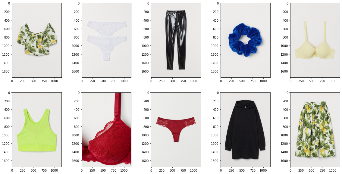
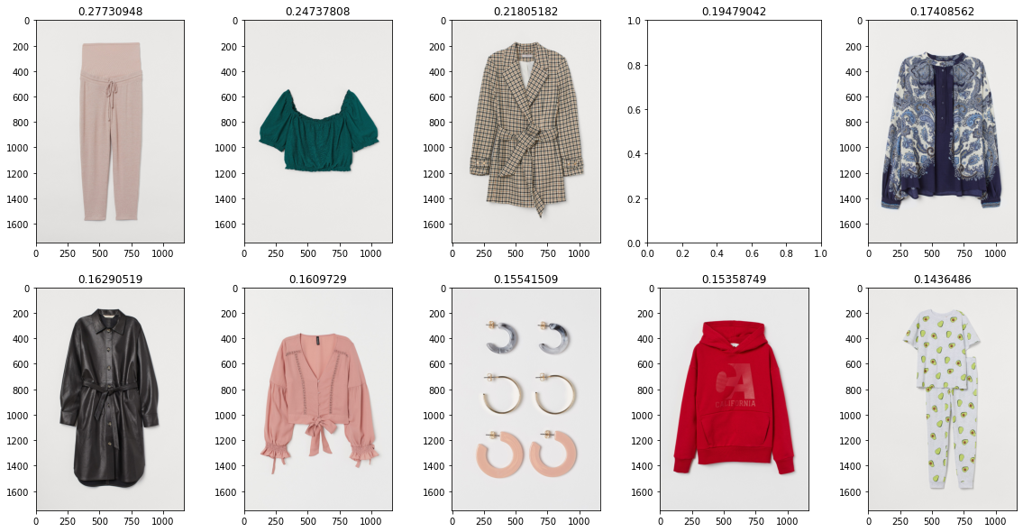
rec_ids, rec_scores = als.recommend(167, purchases_sparse[167])
# Plot purchases vs recs
compare_purchases_and_recs(167, rec_ids, rec_scores, idx_to_user, idx_to_article, purchases_dense, all_files)
And below is the output - the first selection of images are a sample of the users purchases and the second images are the top 10 recommendations.
### Testing the Model
Now we know we’ve got some recommendations that would appear to make sense, we need to test our model on our testing set we create earlier.
Firstly, we can get the recommendations for all of our test users from out model.
recs, scores = als.recommend(
    user_index, # Pass our list of test users
    train[user_index], # Pass the list of all users and their purchases
    filter_already_liked_items=False,
    N=12 # We'll be using Precision@12 so return 12 recs
)
Now we have our recommendations, we can test the scores on both the train and test sets and evaulate it’s performance.
# List to store the scores for each user
test_scores = []
train_scores = []
for i, user in enumerate(user_index):
    train_true_purchases = train.getrow(user).indices
    test_true_purchases = test.getrow(user).indices
    rec_purchases = top_12[i]

    test_score = float(len(set(test_true_purchases) & set(rec_purchases))) / 5.0
    test_scores.append(test_score)

    train_score = float(len(set(train_true_purchases) & set(rec_purchases))) / 5.0
    train_scores.append(train_score)

    print(np.mean(test_scores))
    print(np.mean(train_scores))

>>> 0.03312111549478463
>>> 0.4960082148840729
And we can see that roughly 1 in every 30 of our recommendations was purchased in the subset of user-items in our test set which would appear to be within a similar ball park to the number reported in the tests Ethan Rosenthal ran on a different dataset. The ALS model could be optimised further by assessing the number of training iterations or the number of latent factors.
Purchase Confidence
There is another way we can try to improve our recommendations - improve the accuracy of our confidence values. The initial value for our model was just a 1 where a user purchased an item or a zero otherwise. Let’s look at two possible ways we could do this differently.
- We assume that more recent purchases are more relevant and assign these more weight. We’ll experiment with a 6 month and 12 month window.
def assign_confidence_recent(date):
    if date >= dt.date(2020,3,20):
        return 5
    elif (date >= dt.date(2020,3,20)) & (date < dt.date(2020,3,20)):
        return 3
    else:
        return 1

purchases_dense['confidence_recent'] = purchases_dense['t_dat'].apply(assign_confidence)
- We could assume that recent purchases are most relevant, and that purchases within the same season may be related (i.e. user preferences during autumn/winter may show different correlations to spring/summer. Given our predictions are for September, add more weight for autumn/winter) with all other purchases showing lower confidence.
def assign_confidence(date):
    if date >= dt.date(2020,6,20):
        return 5
    elif date.month in (7,8,9):
        return 3
    else:
        return 1

purchases_dense['confidence'] = purchases_dense['t_dat'].apply(assign_confidence)
But the big question if how do these perform? Models were trained in the exact same way as before with however the sparse user-item matrices were re-created using these new confidence values. Here are the output.
>>> Option 1 Test Accuracy = 0.10464681403015727
>>> Option 1 Train Accuracy = 0.4873544830568015

>>> Option 2 Test Accuracy = 0.10463168134897044
>>> Option 2 Train Acuracy = 0.4876938874777064
Both options perform almost identically and both options perform almost 3 times better than our original model with no confidence weighting at all so it’s a win for our updated confidence values.
Closing Remarks
Collaborative filtering is usually the first stop for insightful recommendations so hopefully this post has shed a little bit of light on how this can be done with implicit feedback data. In the coming posts we’ll look at using cypher queries to create recommendations and how we can combine all these different techniques to get an overall recommendation system working.