
So in the past couple of weeks a Kaggle challenge has been opened up with the task of creating clothing recommendations based on a dataset from H&M. The data consists of images of all the items, user info and item info. Over the course of the next few weeks I’ll be looking at how we can combine multiple different methodologies to create insightful recommendations. I’ll start in this post by loading the data into a Neo4j database and doing some exploratory data analysis and in subsequent posts look at how we can use graph databases for recommendations and how we can incorporate the image data using image embeddings from pre-trained neural networks.
Loading the data
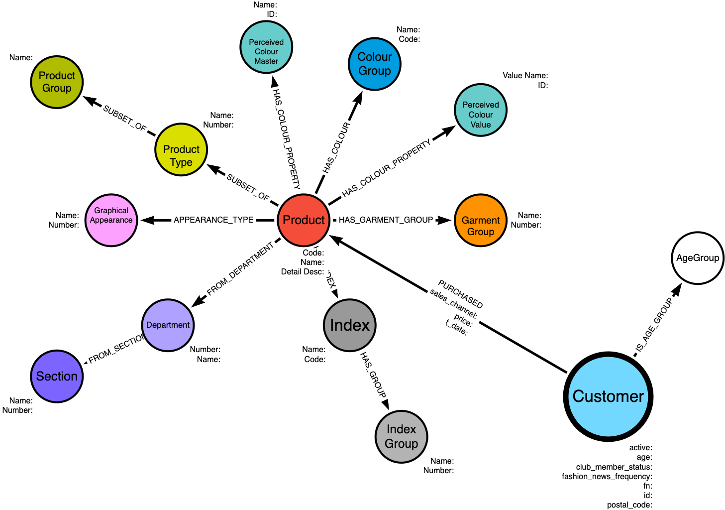
The data can be loaded into a neo4j database using this script. The resulting data model should look something like this:
Exploratory Analysis
import pandas as pd
import numpy as np
from neo4j import GraphDatabase

uri = "bolt://localhost:7687"
driver = GraphDatabase.driver(uri, auth=("neo4j", "password"))
Firstly, let’s get an idea of the number of some summary statistics such as number of customers, number of products and average number of purchases
with driver.session() as session:
    query = """
    MATCH (c:Customer)
    RETURN 'Customer' as Label, COUNT(c) as total_count
    UNION
    MATCH (p:Product)
    RETURN 'Product' as Label, COUNT(p) as total_count
    UNION
    MATCH (c:Customer)-[pur:PURCHASED]->(p:Product)
    RETURN 'Purchases' as Label, COUNT(pur) as total_count
    """

    data = list(session.run(query))

df = pd.DataFrame([dict(record) for record in data])
| Label | total_count | |
|---|---|---|
| 0 | Customer | 1371980 |
| 1 | Product | 105542 |
| 2 | Purchases | 28813419 |
Now we have an idea of the number of user, products and purchases, we can look some other summary statistics such as the average number of purchases per user and the average number of times each item has been purchased
with driver.session() as session:
    query = """
    MATCH (c:Customer)-[pur:PURCHASED]->(p:Product)
    WITH c, COUNT(pur) AS num_purchases
    RETURN
      'Customer Purchases' as Label,
      AVG(num_purchases) as avg,
      stDevP(num_purchases) as std_dev
    UNION
    MATCH (p:Product)<-[pur:PURCHASED]-(c:Customer)
    WITH p, COUNT(pur) AS times_purchased
    RETURN
      'Product Purchased' as Label,
      AVG(times_purchased) as avg,
      stDevP(times_purchased) as std_dev
    """

    data = list(session.run(query))

df = pd.DataFrame([dict(record) for record in data])
| Label | avg | std_dev | |
|---|---|---|---|
| 0 | Customer Purchases | 21.1509 | 34.5904 |
| 1 | Product Purchased | 275.603 | 696.874 |
And now we can see the summary stats for purchases with an average of just over 21 purchases per customer, albeit with a large standard deviation and each item purchased on average 275 times with a huge standard deviation. Looking at the stats I would assume the data is heavily skewed so we can visualise it to find out
with driver.session() as session:
    query = """
    MATCH (c:Customer)-[pur:PURCHASED]->(p:Product)
    WITH c, COUNT(pur) AS num_purchases
    RETURN collect(num_purchases) as purchases
    UNION
    MATCH (p:Product)<-[pur:PURCHASED]-(c:Customer)
    WITH p, COUNT(pur) AS times_purchased
    RETURN collect(times_purchased) as purchases
    """

    data = list(session.run(query))

customer_purchases = data[0][0]
product_purchases = data[1][0]
import seaborn as sns
import matplotlib.pyplot as plt
sns.set_style('whitegrid')


fig, (ax1, ax2) = plt.subplots(figsize=(12,6), ncols=2)
ax1.set_title('Distribution of number of user purchase')
ax2.set_title('Distribution of number of times item purchased')
sns.kdeplot(customer_purchases, ax = ax1)
sns.kdeplot(product_purchases, ax = ax2)
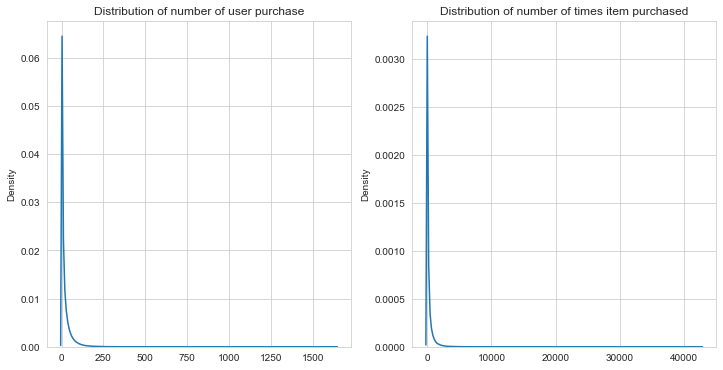
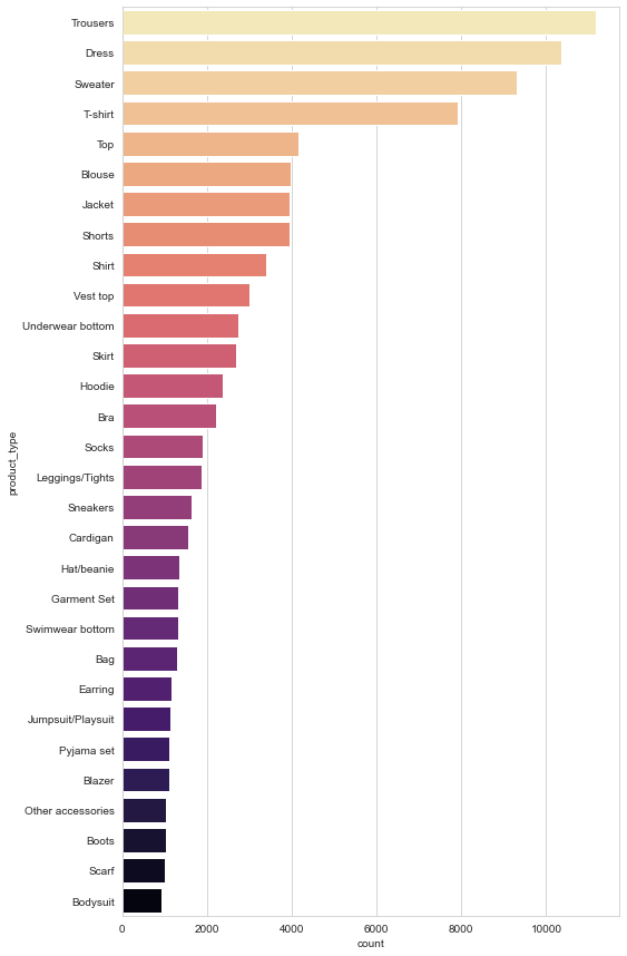
As we can see, the data is massively right skewed meaning we have a small number of users that purchases lots of items with lots of users who purchase only a smaller number of items in comparison and the same for the product distribution. The data model also includes a number of properties relating to the product type so lets explore these next. Firstly we’ll look at the number of products by product type.
with driver.session() as session:
    query = """
    MATCH (p:Product)-[:SUBSET_OF]->(n:ProductType) RETURN n.name as product_type, COUNT(p) as count
    """

    data = list(session.run(query))

df = pd.DataFrame([dict(record) for record in data])

# Save the top product types for later
top_prods = df.sort_values('count', ascending=False).head(30)['product_type']
# Let's have a look at the top 30 types of item
plt.figure(figsize = (8,15))
sns.barplot(
    x='count',
    y='product_type',
    data=df.sort_values('count', ascending=False).head(30),
    palette='magma_r',
)
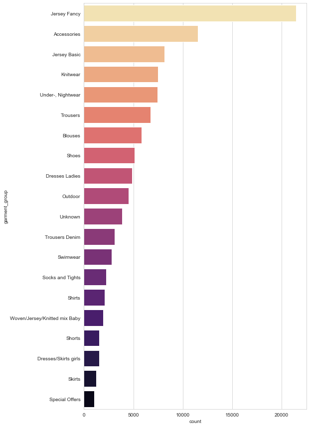
Next, we will look at the number of products divided into their respective garment groups.
with driver.session() as session:
    query = """
    MATCH (p:Product)-[:HAS_GARMENT_GROUP]->(g:GarmentGroup) RETURN g.name as garment_group, COUNT(g) as count
    """

    data = list(session.run(query))

df = pd.DataFrame([dict(record) for record in data])

plt.figure(figsize = (8,15))
sns.barplot(
    x='count',
    y='garment_group',
    data=df.sort_values('count', ascending=False).head(20),
    palette='magma_r'
)
Seasonal Effects
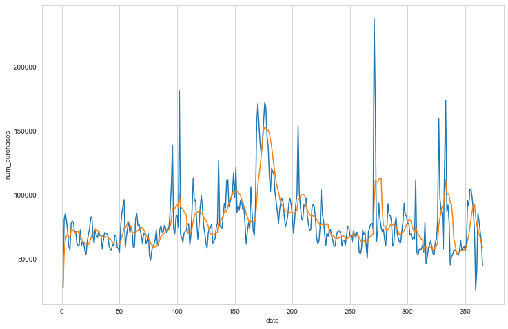
One aspect we haven’t touched on so far is the temporal nature of purchases. Firstly, let’s see how the number of all purchases varies on a daily and weekly basis.
with driver.session() as session:

    query = """
    MATCH ()-[p:PURCHASED]-()
    RETURN p.t_date as date, COUNT(p) as num_purchases
    """

    data = list(session.run(query))

df = pd.DataFrame([dict(record) for record in data])

# Convert neo4j.dates to python datetimes
import datetime as dt
df['date'] = df['date'].apply(lambda x: dt.date(x.year, x.month, x.day))
df['date'] = pd.to_datetime(df['date'])
df.set_index('date', inplace=True)

daily_counts = df.groupby(df.index.dayofyear).mean()

plt.figure(figsize = (12,8))
sns.lineplot(
    x=daily_counts.index,
    y='num_purchases',
    data=daily_counts,
    palette='mako'
)
sns.lineplot(
    x=daily_counts.index,
    y='num_purchases',
    data=daily_counts.rolling(7, min_periods=1).mean(),
    palette='mako'
)
The dataset spans a number of years so I’ve avergaed the count of purchases by the day of the year.
The next question to answer is does this seasonality vary depending on the type of product being purchased?
with driver.session() as session:
    query = """
    MATCH ()-[pur:PURCHASED]->(p:Product)-[:SUBSET_OF]->(n:ProductType)
    RETURN
      pur.t_date as date,
      n.name as product_type,
      COUNT(pur) as count
    """

    data = list(session.run(query))

df = pd.DataFrame([dict(record) for record in data])

df['date'] = df['date'].apply(lambda x: dt.date(x.year, x.month, x.day))
df['date'] = pd.to_datetime(df['date'])
df.set_index('date', inplace=True)

daily_counts = df.groupby([df.index.dayofyear, 'product_type']).mean()
daily_counts daily_counts.reorder_levels([1,0])

plt.figure(figsize = (12,8))

for prod in bestsellers[:10]:
    sns.lineplot(
        x=daily_counts.loc[pd.IndexSlice[:, prod],:].index.get_level_values(0),
        y='count',
        data=daily_counts.loc[pd.IndexSlice[:, prod],:],
        label=prod
     )

plt.legend()
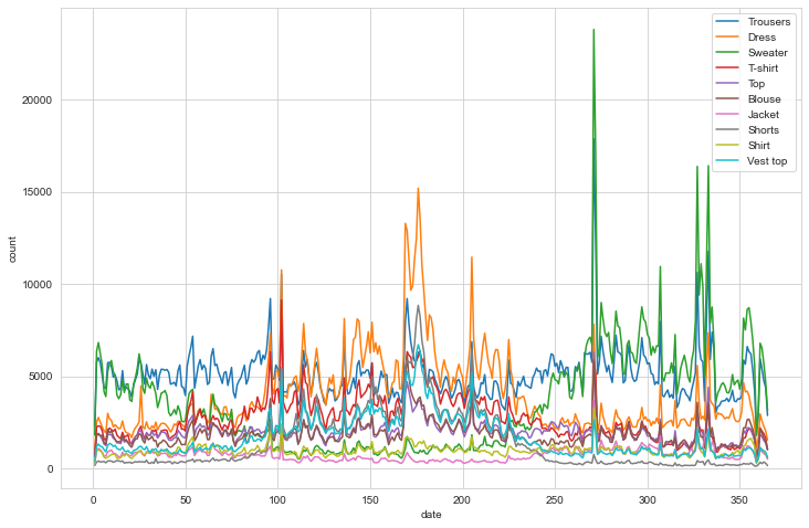
So we can see a few products have slightly different seasonal trends with sweaters, trousers and jackets more popular in the winter months and dresses and t-shirts more popular in Summer…which we probably could have guessed but it’s good to verify and make sure we test any of our assumptions.
Demographic Patterns
Finally, we’ll look at the purchasing patterns by age demographic. Does the type of product purchased vary depending on the customer age?
with driver.session() as session:


    query1 = """
    MATCH (p:Product)-[:SUBSET_OF]->(n:ProductType)
    WITH id(n) as top_products, COUNT(p) as count_prods ORDER BY COUNT(p) DESC LIMIT 30
    WITH collect(top_products) as top_30
    MATCH (a:AgeGroup)<-[:IS_AGE_GROUP]-(:Customer)-[pur:PURCHASED]->(:Product)-[:SUBSET_OF]->(pt:ProductType) WHERE id(pt) IN top_30
    RETURN a.lower as lower, a.upper as upper, COUNT(pur) as total_purchases
    """

    total_by_age = list(session.run(query1))

    query2 = """
    MATCH (p:Product)-[:SUBSET_OF]->(n:ProductType)
    WITH id(n) as top_products, COUNT(p) as count_prods ORDER BY COUNT(p) DESC LIMIT 30
    WITH collect(top_products) as top_30
    MATCH (a:AgeGroup)<-[:IS_AGE_GROUP]-(:Customer)-[pur:PURCHASED]->(:Product)-[:SUBSET_OF]->(pt:ProductType) WHERE id(pt) IN top_30
    WITH a.lower as lower, a.upper as upper, pur, pt.name as product_type
      RETURN
        lower,
        upper,
        product_type,
        COUNT(pur) as num_prod_purchases
    """

    total_by_age_product = list(session.run(query2))
We can then join the two queries together using pandas merge function, pivot the dataframe and plot this on a heatmap to see how product purchases vary by age. Note that some users didn’t have an age in the dataset so these customers were assigned 100 for the age value to keep them separate.
# Join the two dataframes and calculate the proportions
df_total = pd.DataFrame([dict(record) for record in total_by_age])
df_prod = pd.DataFrame([dict(record) for record in total_by_age_product])
df_all = pd.merge(df_total, df_prod, how='inner', on=['lower', 'upper'])
df_all['prod_proportion'] = df_all['num_prod_purchases'] / df_all['total_purchases']

# Pivot the dataframe so it can be plotted as a heatmap
df_pivot = pd.pivot(df_all, 'lower', 'product_type', 'prod_proportion')

plt.figure(figsize = (8,12))
sns.heatmap(df_pivot.T*100, annot=df_pivot.T.values*100)
plt.xlabel('Lower Age')
plt.xlabel('Product Type')
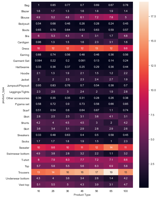
So what can we take away from the data in the heatmap? Relatively speaking as all proportions are relative to the age group :
- Vest tops, bras, playsuits, leggings, shorts and swimwear and underwear bottoms get less popular with age
- Trousers, sweaters, dresses and blouses get more popular with age
Hopefully these bits of info will come in useful when we start looking at how we make recommendations. Next week we’ll look at making recommendations based on the graph alone, followed by using image embeddings and collaborative filtering using implicit data.