To recap last weeks post, we finished by extracting all the named entities from the research paper abstracts and writing them to our graph. A question from Mark Fallu (@brisvegas1) on Twitter after part 1 of this series was interested if we could align graph embeddings with document embeddings so that’s what we’ll explore this week.
Hugging Face Embeddings
Hugging Face makes it almost too easy to transform sentences into embeddings. A quick excerpt from the docs shows just how easy it is…
from sentence_transformers import SentenceTransformer
model = SentenceTransformer('all-MiniLM-L6-v2')

#Our sentences we like to encode
sentences = ['This framework generates embeddings for each input sentence',
    'Sentences are passed as a list of string.',
    'The quick brown fox jumps over the lazy dog.']

#Sentences are encoded by calling model.encode()
embeddings = model.encode(sentences)
So let’s dive in and see how we can run this on our own data.
First of all, create the embeddings after querying the graph.
from sentence_transformers import SentenceTransformer
model = SentenceTransformer('paraphrase-MiniLM-L6-v2')

with driver.session() as session:

    paper_list = list(session.run('MATCH (p:Paper) WHERE EXISTS (p.abstract) RETURN p.title, p.abstract LIMIT 1000'))

paper_abstracts =[abstract['p.abstract'] for abstract in paper_list]
paper_titles = [title['p.title'] for title in paper_list]

#Our sentences we would like to encode
model.max_seq_length = 512

#Sentences are encoded by calling model.encode()
embeddings = model.encode(paper_abstracts)
Next, we can calculate the similarities between all pairs of embeddings.
# Helper function to create all pairwise similarities between embeddings
def cosine_sim(matrix):

    dot = np.dot(matrix, matrix.T)
    norm = np.linalg.norm(matrix, axis=1)
    sim = dot / np.power(norm,2)

    return sim

# Calculate the similarities
embedding_sim = cosine_sim(embeddings)

# Extract the indices of the papers with a similarity > 0.9
# Find similar paper above threshold
most_similar_abstracts = np.argwhere(embedding_sim > 0.95)

# Print some examples, ensuring to filter out rows where both items are
# the same
for row in most_similar_abstracts[most_similar_abstracts[:,0] != most_similar_abstracts[:,1]]:
    print(f'\n------- SCORE: {embedding_sim[row[0], row[1]]}')
    print(paper_titles[row[0]])
    print(paper_titles[row[1]])

>> ------- SCORE: 0.9643388986587524
>> Pretesting static and dynamic stretching does not affect maximal strength
>> Acute effects of static and ballistic stretching on measures of strength and power

>> ------- SCORE: 0.9921305179595947
>> The duration of the inhibitory effects with static stretching on quadriceps peak torque production
>> Acute effects of static and ballistic stretching on measures of strength and power

>> ------- SCORE: 0.9926120638847351
>> Monitoring exercise intensity during resistance training using the session RPE scale
>> Session Rating of Perceived Exertion as an Efficient Tool for Individualized Resistance Training Progression
And we can see that the similarity scores make sense when looking at the title of the most similar pairs of papers. Good start for Hugging Face.
If we reduce the dimensionality of the embeddings with TSNE and visualize them, we can begin to get an idea of where some of these papers sit relative to each other and how they cluster together.
from sklearn.manifold import TSNE
import altair as alt

X_embedded = TSNE(n_components=2, random_state=6).fit_transform(embeddings)

df = pd.DataFrame(data={
    'abstract': paper_abstracts,
    'title': paper_titles,
    'x': [x[0] for x in X_embedded],
    'y': [x[1] for x in X_embedded]
})

alt.Chart(df).mark_circle(size=60).encode(
    x='x',
    y='y',
    tooltip=['title']
).properties(width=700, height=400)
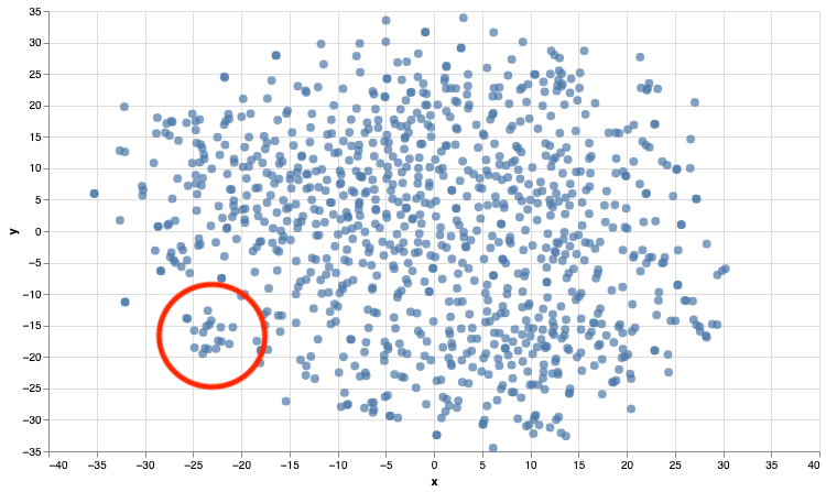
If we have a look at a cluster of papers highlighted in the red circle, it’s fairly obvious that we’re starting to get clusters based on the topics of the papers…
| Titles |
|---|
| ‘Physiological responses of simulated karate sparring matches in young men and boys’ |
| ‘Assessment of maximal cardiorespiratory performance and muscle power in the Italian Olympic judoka’ |
| ‘Cardiovascular response to punching tempo’ |
| ‘Is Bilateral Deficit in Handgrip Strength Associated With Performance in Specific Judo Tasks?’ |
| ‘Early Signs of Inflammation With Mild Oxidative Stress in Mixed Martial Arts Athletes After Simulated Combat’ |
| ‘Physiological Responses During Female Judo Combats: Impact of Combat Area Size and Effort to Pause Ratio Variations’ |
| ‘Physiological Responses and Time-Motion Analysis of Kickboxing: Differences Between Full Contact, Light Contact, and Point Fighting Contests’ |
| ‘Exercise Response to Real Combat in Elite Taekwondo Athletes Before and After Competition Rule Changes’ |
| ‘Validity of an Interval Taekwondo-Specific Cardiopulmonary Exercise Test’ |
| “Effects of High-Intensity Interval Training on Olympic Combat Sports Athletes’ Performance and Physiological Adaptation: A Systematic Review” |
| ‘Physiological and Biomechanical Responses to an Acute Bout of High Kicking in Dancers’ |
| ‘Can Caffeine Intake Improve Neuromuscular and Technical-Tactical Performance During Judo Matches?’ |
| ‘Effects of Judo Training on Bones: A Systematic Literature Review’ |
| ‘Effect of Postactivation Potentiation Induced by Elastic Resistance on Kinematics and Performance in a Roundhouse Kick of Trained Martial Arts Practitioners’ |
| ‘Rating of Perceived Exertion for Quantification of Training and Combat Loads During Combat Sport-Specific Activities: A Short Review’ |
| ‘Mixed Martial Arts Induces Significant Fatigue and Muscle Damage Up to 24 Hours Post-combat’ |
| ‘Physiological Responses and Time-Motion Analysis of Small Combat Games in Kickboxing: Impact of Ring Size and Number of Within-Round Sparring Partners’ |
| ‘Physical and Physiological Attributes of Wrestlers: An Update’ |
### Author Embeddings
One are that I’ve found interesting is how we can average a collection of embeddings - for example, some people would average a collection of word embeddings to create a sentence embedding. In a similar vein, I thought it would be interesting see if we can create and Author embedding based on averaging the sentence embeddings derived from their paper abstracts. This article suggests it’s doable and the author sounds like he knows what he’s talking about…certainly more than me anyway!
## top_auth was created from the highest ranked authors in an earlier port

 with driver.session() as session:

    author_papers = list(session.run('MATCH (p:Paper)-[:AUTHORED]-(a:Author) WHERE a.name IN \
    $authors and exists (p.abstract) RETURN a.name as name, p.abstract as abstract', {'authors':top_auth.tolist()}))

# Create dataframe from data
df_auth = pd.DataFrame([dict(record) for record in author_papers])

#Our sentences we like to encode
model.max_seq_length = 512

#Sentences are encoded by calling model.encode()
embeddings = model.encode(df_auth['abstract'].values)

# Extract all unique authors
authors = df_auth['name'].unique()
avg_embeddings = {}

# Take and average embedding for each author
for auth in authors:
    avg_embeddings[auth] = embeddings[df_auth['name'] == auth].mean(axis=0)

# Convert to a dataframe
avg_embedding_df = pd.DataFrame(avg_embeddings).T

# Reduce dimensions for visualization
X_embedded = TSNE(n_components=2, random_state=6).fit_transform(avg_embedding_df.values)

# Plot with labels
df = pd.DataFrame(data={
    'name': avg_embedding_df.index,
    'x': [x[0] for x in X_embedded],
    'y': [x[1] for x in X_embedded]
})

points = alt.Chart(df).mark_circle(size=60).encode(
    x='x',
    y='y',
    tooltip=['name']
).properties(width=700, height=400)

text = points.mark_text(
    align='left',
    baseline='middle',
    dx=7
).encode(
    text='name'
)

points + text
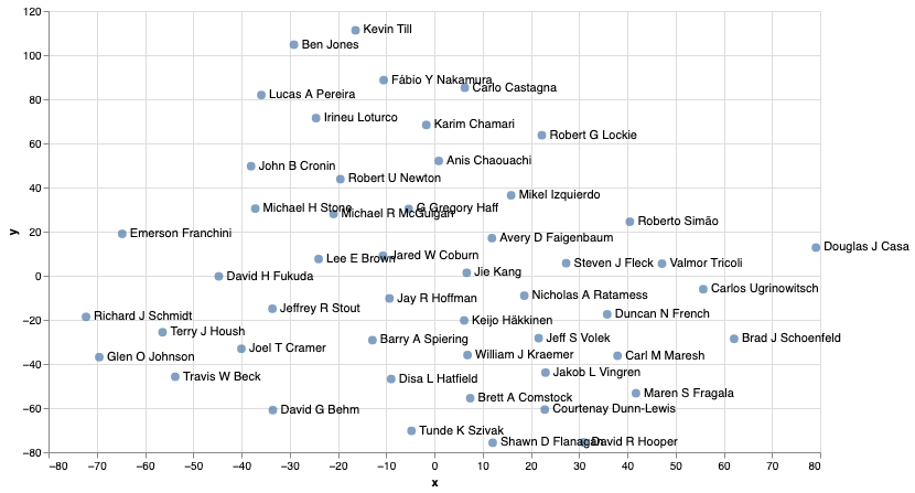
And from this we can see that authors with similar research interests end up quite close in the embedding space.
Graph Embeddings from Named Entities
Finally, we will look at how we can create embeddings from our graph. First off we will create the graph projection with Authors, Papers and Entity nodes and then we’ll create the embeddings from this graph projection.
with driver.session() as session:

    session.run("""
    CALL gds.graph.create(
      'ner_embeddings',
      ['Paper', 'Entity','Author'],
      {
        ENTITY: {
          orientation: 'UNDIRECTED'
        },
        AUTHORED: {
          orientation: 'UNDIRECTED'
        }
      }
    )
    """)

    ner_embeddings = list(session.run("""
    CALL gds.fastRP.stream(
      'ner_embeddings',
      {
        embeddingDimension: 128
      }
    )
    YIELD nodeId, embedding
    WITH nodeId, gds.util.asNode(nodeId) AS paper, embedding WHERE paper:Paper
    RETURN nodeId, paper.title as paperTitle,
    embedding
    """, ))

# Create two lists for titles and embeddings and pass to dataframe
ner_title = [paper['paperTitle'] for paper in ner_embeddings]
ner_embeddings = [paper['embedding'] for paper in ner_embeddings]

ner_df = pd.DataFrame(
    data = {
        'title': ner_title,
        'embedding': ner_embeddings
    }
)
The embeddings have been calculated and stored in a pandas DataFrame. We can now compute similarities between each Paper.
ner_embedding_sim = cosine_sim(np.asarray(ner_embeddings))
similar_ner_embeddings = np.argwhere(ner_embedding_sim > 0.95)

for row in similar_ner_embeddings[similar_ner_embeddings[:,0] != similar_ner_embeddings[:,1]]:
    print(f'\n----- SCORE: {ner_embedding_sim[row[0], row[1]]}')
    print(ner_title[row[0]])
    print(ner_title[row[1]])


----- SCORE: 0.9558417405891849
Short-term effect of strength training with and without superimposed electrical stimulation on muscle strength and anaerobic performance. A randomized controlled trial. Part I
Short-term effect of plyometrics and strength training with and without superimposed electrical stimulation on muscle strength and anaerobic performance: A randomized controlled trial. Part II

----- SCORE: 0.9880140540149642
Mechanomyographic and electromyographic responses during submaximal to maximal eccentric isokinetic muscle actions of the biceps brachii
Mechanomyographic and electromyographic responses of the vastus medialis muscle during isometric and concentric muscle actions

----- SCORE: 0.9656198996657351
Physiological and anthropometric characteristics of junior rugby league players over a competitive season
Changes in physiological and anthropometric characteristics of rugby league players during a competitive season

----- SCORE: 0.9582480082449912
Effects of Combined Resistance Training and Weightlifting on Motor Skill Performance of Adolescent Male Athletes
Effects of Combined Resistance Training and Weightlifting on Injury Risk Factors and Resistance Training Skill of Adolescent Males

----- SCORE: 0.9677283350042296
Assessing Repeated-Sprint Ability in Division I Collegiate Women Soccer Players
Repeated-Sprint Ability in Division I Collegiate Male Soccer Players: Positional Differences and Relationships With Performance Tests
Using these embeddings we get some pretty good similarities between papers which also make sense when looking at the titles.
Author Embeddings - Return of the Graph
Now we’ll repeat the same averaging of Paper embeddings to see if we can create a reasonable representation of an Author.
with driver.session() as session:

    avg_auth = list(
        session.run(
            """MATCH (a:Author)-[:AUTHORED]->(p:Paper)
            RETURN id(a), a.name, p.title, p.embedding as embedding
            """
        )
    )

avg_auth = pd.DataFrame([dict(record) for record in avg_auth])

avg_embedding = avg_aut.groupby('a.name')['embedding'].apply(lambda x: np.vstack(x).mean(axis=0))

avg_embedding = avg_embedding[avg_embedding.index.isin(top_auth)]

X_embedded = TSNE(n_components=2, random_state=6).fit_transform(avg_embedding.tolist())

df = pd.DataFrame(data={
    'name': avg_embedding.index,
    'x': [x[0] for x in X_embedded],
    'y': [x[1] for x in X_embedded]
})

points = alt.Chart(df).mark_circle(size=60).encode(
    x='x',
    y='y',
    tooltip=['name']
).properties(width=700, height=400)

text = points.mark_text(
    align='left',
    baseline='middle',
    dx=7
).encode(
    text='name'
)

points + text
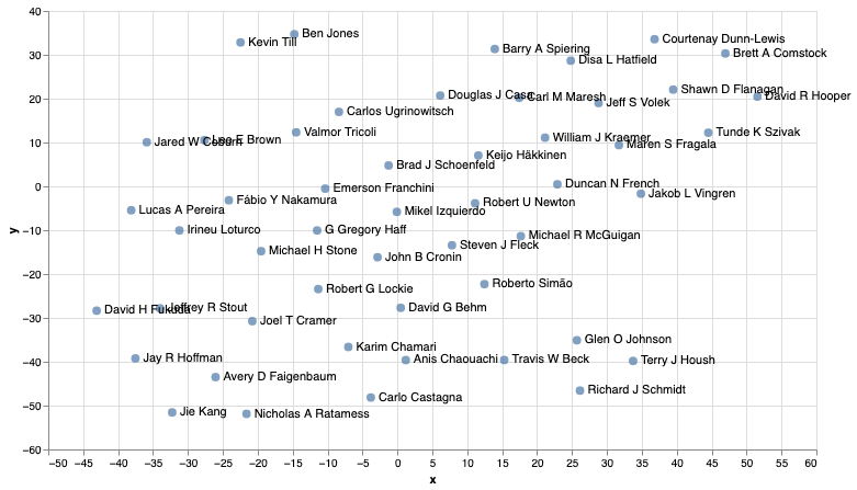
And if you take the time to peruse both graphs, you’ll see that in most cases the authors are represented within a similar area in both graphs which I think is quite interesting given the two different approaches to calculating the embeddings.