In last weeks post, we loaded up a graph with research papers and the associated authors and institutions. This week we’ll look at a few different things:
- Using the Neo4j GDS library to run some analysis on the graph.
- Using named entity recognition to extract entities from the paper abstracts and create nodes for these entities.
- Computing embeddings for various aspects of the graph and comparing these to some other embedding methods.
Centrality
One way to analyse the graph is to examine the centrality of the nodes - this is a way to determine the importance of distinct nodes in a network. When looking at research papers, one of the easiest ways to determine the importance of a paper would be to use a PageRank or more likely Article Rank type algorithm as these are specifically designed for this use case - essentially a paper is only as important as the papers that reference it. In our case, when we’re looking at authors of these papers, we can look at Degree centrality based on the number of co-authors. Lets see how this would look to code up. We’ll start by connecting to our database:
from neo4j import GraphDatabase

uri = "bolt://localhost:7687"
driver = GraphDatabase.driver(uri, auth=("neo4j", "password"))
And next we need to create our graph projection, creating the relationship with a count of how many papers have been co-authored:
with driver.session() as session:
    session.run("""
    CALL gds.graph.create.cypher(
    'coAuthors',
    'MATCH (a:Author) RETURN id(a) as id, labels(a) as labels',
    'MATCH (a1)-[:AUTHORED]->(p:Paper)<-[:AUTHORED]-(a2)
     WHERE id(a1) > id(a2)
     RETURN id(a1) AS source, id(a2) as target, COUNT(p) as coPapers'
    )
    YIELD
    graphName AS graph, nodeCount AS nodes, relationshipCount AS rels
"""
    )
The next step is to run the algorithm and write the results back to the graph.
with driver.session() as session:

    session.run(
        """
        CALL gds.degree.write(
            'coAuthors',
            {
                relationshipWeightProperty: 'coPapers',
                orientation: 'UNDIRECTED',
                writeProperty: 'degree_score'
            }
        )
        YIELD nodePropertiesWritten
        RETURN nodePropertiesWritten
        """
    )

    degree = list(session.run(
        """
        MATCH (a:Author)
        RETURN a.name as name, a.degree_score as score
        ORDER BY score DESC
        """
    ))

df = pd.DataFrame([dict(record) for record in degree])

|       | name                |   score |
|------:|:--------------------|--------:|
| 12388 | William J Kraemer   |     855 |
| 12398 | Carl M Maresh       |     556 |
| 12397 | Jeff S Volek        |     547 |
| 12665 | Robert U Newton     |     429 |
| 12393 | Nicholas A Ratamess |     418 |
| 12564 | Lee E Brown         |     415 |
| 12214 | Keijo Häkkinen      |     415 |
| 12498 | Mikel Izquierdo     |     377 |
| 12698 | Jay R Hoffman       |     362 |
And looking at the table, the results would make sense as these researchers would be some of the most prominent. However as quick sanity check, we can run a simple query to see which authors have the most co-authors.
with driver.session() as session:
    coAuthor = list(
            session.run(
            """
            MATCH (a1:Author)-[:AUTHORED]->(p:Paper)<-[:AUTHORED]-(a2:Author)  WHERE id(a1) <> id(a2)
            RETURN a1.name as name, COUNT(DISTINCT a2) as countCo ORDER BY countCo DESC
            """
            )
    )

df_co = pd.DataFrame([dict(record) for record in coAuthor])
|    | name                |   countCo |
|---:|:--------------------|----------:|
|  0 | William J Kraemer   |       311 |
|  1 | Mikel Izquierdo     |       215 |
|  2 | Robert U Newton     |       204 |
|  3 | Lee E Brown         |       201 |
|  4 | Keijo Häkkinen      |       174 |
|  5 | Nicholas A Ratamess |       172 |
And although not perfectly aligned, we can see that the degree centrality score would make sense.
Flow of Information
Betweenness centrality is a way of detecting the amount of influence a node has over the flow of information in a graph. It is often used to find nodes that serve as a bridge from one part of a graph to another.
Using the betweenness centrality algorithm, we can use the same graph projection to see which nodes have the most influence over the flow of information in the graph.
 with driver.session() as session:
    flow = list(
        session.run(
            """
            CALL gds.betweenness.stream('coAuthors')
            YIELD nodeId, score
            RETURN gds.util.asNode(nodeId).name AS name, score
            ORDER BY score DESC
            """
        )
    )
df_flow = pd.DataFrame([dict(record) for record in flow])

|    | name                 |   score |
|---:|:---------------------|--------:|
|  0 | Robert U Newton      |  858602 |
|  1 | William J Kraemer    |  738341 |
|  2 | G Gregory Haff       |  690774 |
|  3 | Mikel Izquierdo      |  679513 |
|  4 | Emerson Franchini    |  578170 |
|  5 | Brad J Schoenfeld    |  536420 |
And as we can see above, some of the researchers with the most co-authors come out on top but not the case for everyone. Those that form the link between mulitple research groups may be the ones who control the largest flow of information between the nodes.
Embeddings
Excuse the Despicable Me reference, but embeddings are just reducing the dimensionality of our graph structure whilst preserving as much information as possible from our graph structure in an N-dimensional vector which has…

We’ll start by using the FastRP algorithm and although the docs suggest it can only be ran on an homogenous graph projection, the Neo4j forums suggest it can be ran on heterogenous graphs, so we’ll run with it and see what the outcome is. I’d also suggest looking at Zach Blumenfeld’s code for good examples of this
We’ll start by creating a new graph projection based on research papers and their authors.
with driver.session() as session:
    session.run(
        """
        CALL gds.graph.create(
            'embeddings',
            ['Author', 'Paper'],
            {
                AUTHORED:{
                    orientation:'UNDIRECTED'
                }
            }
        ) YIELD nodeCount, relationshipCount, createMillis
        """
    )
Next we can create the embeddings based off the new graph projection.
with driver.session() as session:
    embeddings = session.run(
        """
        CALL gds.fastRP.mutate(
            'embeddings',
            {
                mutateProperty: 'embedding',
                embeddingDimension: 196,
                randomSeed: 7474
            }
        )
        YIELD nodePropertiesWritten, computeMillis
        """
    )

    knn = list(session.run(
        """
        CALL gds.beta.knn.stream(
            'embeddings', {
                nodeWeightProperty: 'embedding'
            }
        )
        YIELD node1, node2, similarity
        WITH gds.util.asNode(node1) as p1, gds.util.asNode(node2) as p2, similarity
        WHERE p1:Paper AND p2:Paper and id(p1) > id(p2)
        MATCH (p1)<-[:AUTHORED]-(a:Author)
        MATCH (p2)<-[:AUTHORED]-(a2:Author)
        RETURN p1.title, p2.title, collect(DISTINCT a.name) as auth1,
        collect(DISTINCT a2.name) as auth2, similarity ORDER BY similarity DESC
        """
    ))
The screenshot below shows a sample of the top results with a similarity score of 1 and we can see that papers authored by the exact same authors have the highest similarity.
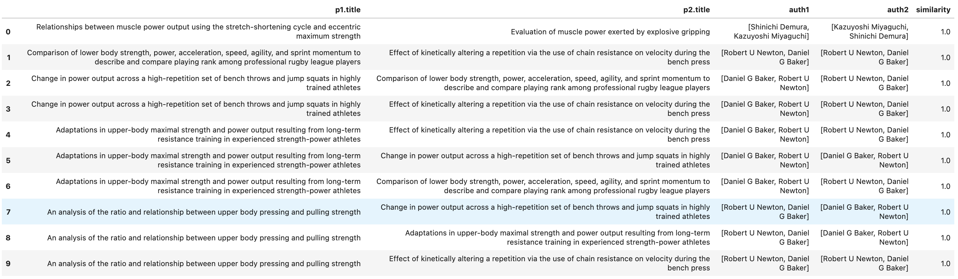
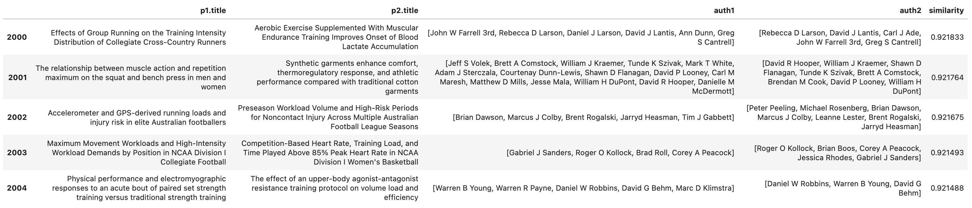
And as we get further down the similarity scores, we can see that the list of authors remains similar but there are some difference.
We can also run a similar query but examine the similarity between authors.
with driver.session() as session:
    knn_auth = list(session.run(
        """
        CALL gds.beta.knn.stream(
            'embeddings', {
                nodeWeightProperty: 'embedding'
            }
        )
        YIELD node1, node2, similarity
        WITH gds.util.asNode(node1) as a1, gds.util.asNode(node2) as a2, similarity
        WHERE a1:Author AND a2:Author and id(a1) > id(a2)
        MATCH (p1:Paper)<-[:AUTHORED]-(a1)
        MATCH (p2:Paper)<-[:AUTHORED]-(a2)
        RETURN a1.name, a2.name, collect(DISTINCT p1.title) as papers1,
        collect(DISTINCT p2.title) as papers2, similarity ORDER BY similarity DESC
        """
    ))
This one is similar to the results above. For people who only have one co-authorship between them, they get a similarity score of 1. If we have people with co-authorships but also papers not co-authored with the other person, then this is where the similarity scores start to reduce. However, I’d question the value of this over a simple jaccard similarity based on a bipartite ‘Author’, ‘Paper’ graph projection.
Named Entity Recognition
To finish this week’s post and lead into Part 3, we’ll extract the entities from each of the paper abstracts and use them to create Entity nodes in the graph. Fortunately there’s some apoc functions which will allow us to do this relatively simply.
Initially I tried batching the query to make parallel requests to the GCP API and avoid memory issues however I still ended up with an error and no entities written to the database.
CALL apoc.periodic.iterate("
  MATCH (p:Paper)
  WITH collect(p) as total
  CALL apoc.coll.partition(total, 25)
  YIELD value as nodes
  RETURN nodes", "
  CALL apoc.nlp.gcp.entities.graph(nodes, {
    key: $apiKey,
    nodeProperty: 'abstract',
    writeRelationshipType: 'ENTITY',
    write:true
  })
  YIELD graph
  RETURN distinct 'done'", {
    batchSize: 1,
    params: { apiKey: $apiKey }
  }
);
Given that batching in this way didn’t work, along with trying various different methods of UNWIND, the next approach was to just call each request one by one for each paper. Probably not the optimal way to do it but it worked in the end.
with driver.session() as session:

    paper_nodes = list(
        session.run(
        """
        MATCH (p:Paper)
        RETURN id(p)
        """
        )
    )

    for node in paper_nodes:
        node_id = node['id(p)']


        session.run(
        """
        WITH $pId as pId, $apiKey as apiKey
        MATCH (p:Paper) WHERE id(p) = pId AND NOT EXISTS((p)-[:ABSTRACT_ENTITY]-()) AND EXISTS (p.abstract)
        CALL apoc.nlp.gcp.entities.graph(p, {
          key: apiKey,
          nodeProperty: 'abstract',
           writeRelationshipType: 'ABSTRACT_ENTITY',
          write:true
          }
        )
          YIELD graph
          RETURN 'done'
        """,
        {'pId': node_id, 'apiKey': apiKey}
        )
And just to show it works…
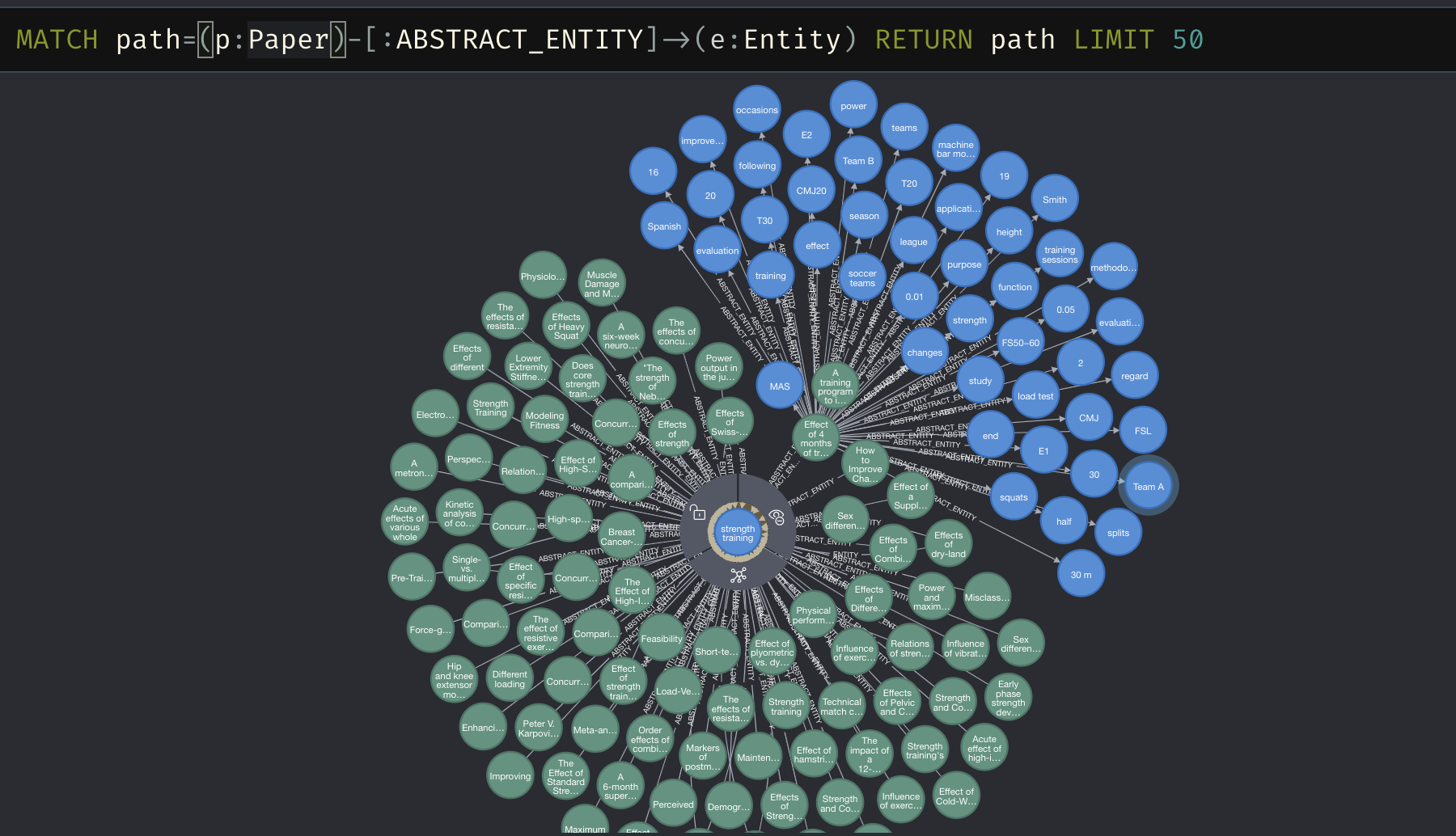
Next week we’ll look at using these entities as part of the embeddings. Until then…