
So I thought I’d do a post for those interested in rugby this week and look at how we can model the number of tries scored per team per game. I’ll look at fetching the data from a database, processing the data and finally what sort of distribution we can use to best model the data. Let’s start with accessing the database.
import mysql.connector
import pandas as pd
import numpy as np
conn = mysql.connector.connect(
    user='user',
    password='password',
    database='db'
)

cur = conn.cursor()
Querying the Database
The aim of the query is to return all of the tries scored and the time in the match that they were scored so we could then calculate the average time period between tries. This sounded simple at first, however I realised I also needed to find a way to return an entry for a team in a fixture even if they didn’t score a try so we could consider the additional 80 minutes between tries scored.
// Select any fixtures between premiership teams
WITH fixtures AS (
  SELECT
    f.fxid,
    f.FxDate
  FROM
    fix_data f
  WHERE
    f.FxHTID IN ( 84,1000,1050,1100,1150,1250,1300,1350,1400,1450,1500,1550,3300)
  AND
    f.FxATID IN ( 84,1000,1050,1100,1150,1250,1300,1350,1400,1450,1500,1550,3300)
)

// Select only tries and the match time they were scored
SELECT
  m.fxid as fxid,
  team_id,
  fixtures.`FxDate`,
  PLID,
  MatchTime,
  `ID`,
  1 as counter
FROM
  match_data m
INNER JOIN
  fixtures
ON
  fixtures.fxid = m.fxid
WHERE EXISTS
  (SELECT
    1
   FROM
    fixtures f
   WHERE
     f.fxid = m.fxid
   )
AND
  action = 9

/* We then need to check for games whereby there wasn't a try scored by a team
and return a dummy entry for this match. We can query with a NOT EXISTS to check
that a try didnt occur in a fixture for a team */

UNION

SELECT DISTINCT
  m.fxid as fxid,
  team_id,
  fixtures.`FxDate`,
  -1 AS PLID,
  9959 AS MatchTime,
  -1 AS `ID` ,
  0 as counter
FROM
  match_data m
INNER JOIN
  fixtures
ON
  fixtures.fxid = m.fxid
WHERE NOT EXISTS (
  SELECT
    fxid,
    team_id
  FROM
    match_data m2
  WHERE
    m2.fxid = fixtures.fxid
  AND
    m2.team_id = m.team_id
  AND
    action = 9
  )
cur.execute(query)
data = cur.fetchall()
df = pd.DataFrame.from_records(data, columns=[x[0] for x in cur.description])
df.head()
| fxid | team_id | FxDate | PLID | MatchTime | ID | counter | |
|---|---|---|---|---|---|---|---|
| 0 | 23312 | 1150 | 2019-03-30 | 28736 | 1601 | 20100663 | 1 |
| 1 | 23312 | 3300 | 2019-03-30 | 11627 | 2318 | 20100751 | 1 |
| 2 | 23312 | 3300 | 2019-03-30 | 20444 | 4559 | 20102079 | 1 |
| 3 | 23312 | 1150 | 2019-03-30 | 10304 | 6907 | 20102962 | 1 |
| 4 | 23638 | 1250 | 2021-04-10 | 30387 | 412 | 25585378 | 1 |
df.fillna(0, inplace=True)

# Sort values by fxid and match time so we have an ordered dataframe
df = df.sort_values(['fxid', 'MatchTime'])
# Calculate the cumulative sum of tries during the game so we have
# tries for at each point during the game
df['try_for'] = df.groupby(['fxid', 'team_id']).cumsum()['counter']
# We can also see an example of when a try wasn't scored
df[df['fxid'] == 118052]
| fxid | team_id | FxDate | PLID | MatchTime | ID | counter | try_for | |
|---|---|---|---|---|---|---|---|---|
| 153 | 118052 | 1500 | 2017-09-29 | 8442 | 539 | 14684544 | 1 | 1 |
| 154 | 118052 | 1500 | 2017-09-29 | 9486 | 5124 | 14685365 | 1 | 2 |
| 155 | 118052 | 1500 | 2017-09-29 | 8442 | 7723 | 14686006 | 1 | 3 |
| 2213 | 118052 | 3300 | 2017-09-29 | -1 | 9959 | -1 | 0 | 0 |
# The next function calculate the total number of tries at each point in the game
# by grouping by fxid and using the cumsum function again
df['cum_try_total'] = df.groupby('fxid').cumsum()['counter']


# Subsequently, we can calculate the tries against at any point in the match as well
df['try_against'] = df['cum_try_total'] - df['try_for']

df[df['fxid'] == 118052]
| fxid | team_id | FxDate | PLID | MatchTime | ID | counter | try_for | cum_try_total | try_against | |
|---|---|---|---|---|---|---|---|---|---|---|
| 153 | 118052 | 1500 | 2017-09-29 | 8442 | 539 | 14684544 | 1 | 1 | 1 | 0 |
| 154 | 118052 | 1500 | 2017-09-29 | 9486 | 5124 | 14685365 | 1 | 2 | 2 | 0 |
| 155 | 118052 | 1500 | 2017-09-29 | 8442 | 7723 | 14686006 | 1 | 3 | 3 | 0 |
| 2213 | 118052 | 3300 | 2017-09-29 | -1 | 9959 | -1 | 0 | 0 | 3 | 3 |
## Matchtime in format mmss but leading zeros missing. Pad with zeros the then convert to TimeDelta
df['MatchTime'] = df['MatchTime'].astype('str').str.pad(width=4, side='left', fillchar='0')

# Add a colon to the match time value
df['MatchTime'] = df['MatchTime'].apply(lambda x: x[:2] + ':' + x[2:])

df['MatchTime']
0       16:01
1       23:18
2       45:59
3       69:07
4       04:12
        ...
2206    36:06
2207    41:32
2208    53:48
2209    56:25
2210    76:50
Name: MatchTime, Length: 2254, dtype: object
The following function converts all the MatchTime strings to a proper datetime, also taking into account the dummy entries for the matches where there was no try for a team.
import datetime
def convert_to_delta(time_string):

    if time_string == '.0':
        delta = datetime.timedelta(hours=1, minutes=20, seconds=0)
        return delta

    if int(time_string[:2]) > 59:
        new_min = int(time_string[:2]) - 60
        new_time = f'01:{new_min}:{time_string[3:]}'
        t = datetime.datetime.strptime(new_time, '%H:%M:%S')
        delta = datetime.timedelta(hours=t.hour, minutes=t.minute, seconds=t.second)

        return delta
    else:

        t = datetime.datetime.strptime(time_string, '%M:%S')
        delta = datetime.timedelta(hours=t.hour, minutes=t.minute, seconds=t.second)

        return delta
# Run the funtion and also convert to seconds
df['MatchTimeDelta'] = df['MatchTime'].apply(convert_to_delta)
df['MatchTimeSeconds'] = df['MatchTimeDelta'] /  np.timedelta64(1, 's')
The next cell applies some if/else logic to calculate the amount of time between tries but also spans the time across multiple games including games whereby there was no try.
all_df = []

for row_num, rows in df.sort_values(['team_id','fxid', 'MatchTime']).groupby(['team_id']):
    match_time_seconds_delta = []
    n_rows = rows.shape[0]

    for idx in range(n_rows):
        if idx == 0 or idx == n_rows:
            match_time_seconds_delta.append(rows.iloc[idx]['MatchTimeSeconds'])
            continue

        elif rows.iloc[idx]['MatchTimeSeconds'] < rows.iloc[idx - 1]['MatchTimeSeconds']:
            seconds =  4800 - rows.iloc[idx - 1]['MatchTimeSeconds'] + rows.iloc[idx]['MatchTimeSeconds']
            match_time_seconds_delta.append(seconds)

        elif rows.iloc[idx]['MatchTimeSeconds'] == 5999.0:
            seconds =  4800 - rows.iloc[idx - 1]['MatchTimeSeconds'] + 4800
            match_time_seconds_delta.append(seconds)

        elif rows.iloc[idx - 1]['MatchTimeSeconds'] == 5999.0:
            seconds = rows.iloc[idx]['MatchTimeSeconds']
            match_time_seconds_delta.append(seconds)

        else:
            seconds =  rows.iloc[idx]['MatchTimeSeconds'] - rows.iloc[idx - 1]['MatchTimeSeconds']
            match_time_seconds_delta.append(seconds)


    rows['MatchSecondsDelta2'] = match_time_seconds_delta
    all_df.append(rows)
# We know the data is sorted, so reset the index and for any fixture/team without a try,
# roll the 80 minutes over into the next try scoring period
for d in all_df:
    d.reset_index(inplace=True)
    no_scores_idx = d[d['ID'] == -1].index
    for idx in no_scores_idx:
        d.loc[idx + 1, 'MatchSecondsDelta2'] += d.loc[idx, 'MatchTimeSeconds']

df = pd.concat(all_df)

df.head()
| level_0 | index | fxid | team_id | FxDate | PLID | MatchTime | ID | counter | try_for | cum_try_total | try_against | MatchTimeDelta | MatchTimeSeconds | MatchSecondsDelta2 | |
|---|---|---|---|---|---|---|---|---|---|---|---|---|---|---|---|
| 0 | 0 | 11 | 118011 | 84 | 2017-09-01 | 20339 | 03:52 | 14394797 | 1 | 1 | 1 | 0 | 0 days 00:03:52 | 232.0 | 232.0 |
| 1 | 1 | 13 | 118011 | 84 | 2017-09-01 | 20339 | 27:55 | 14395376 | 1 | 2 | 3 | 1 | 0 days 00:27:55 | 1675.0 | 1443.0 |
| 2 | 2 | 16 | 118011 | 84 | 2017-09-01 | 19218 | 70:10 | 14400577 | 1 | 3 | 6 | 3 | 0 days 01:10:10 | 4210.0 | 2535.0 |
| 3 | 3 | 67 | 118023 | 84 | 2017-09-09 | 19087 | 10:58 | 14491379 | 1 | 1 | 1 | 0 | 0 days 00:10:58 | 658.0 | 1248.0 |
| 4 | 4 | 68 | 118023 | 84 | 2017-09-09 | 84 | 24:20 | 14491595 | 1 | 2 | 2 | 0 | 0 days 00:24:20 | 1460.0 | 802.0 |
# Convert the times to minutes
df['MatchTimeMinDelta'] = df['MatchSecondsDelta2'] / 60


intervals = [0,10,20,30,40,50,60,70,80,90,float('inf')]

pd.cut(df['MatchTimeMinDelta'], bins=intervals).value_counts().plot(kind='bar')
<AxesSubplot:>
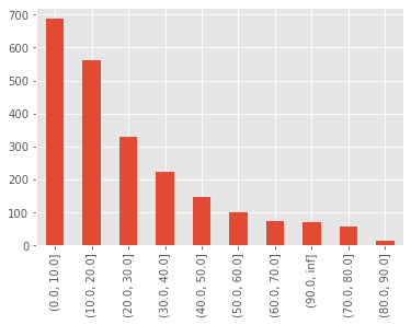
At a brief glance, it appears the timing of tries being scored fits an exponential (geometric if we look at it in discrete bins) distribution. So in reality, the most likely time for a try to be scored after a previous try is within the next 10 minutes. Simple.
Are these tries poisson distributed?
A Poisson distribution models the count of events in a given time period - i.e. $\lambda$ per unit time. In our instance we will look at number of tries per game (80 minutes)
\[p_{X}(x) = \frac{e^{-\lambda}\lambda^x}{x!}\]If Poisson events take place on average at the rate of $\lambda$ per unit of time, then the sequence of time between events are independent and identically distributed exponential random variables, having mean $\beta = \frac{1}{\lambda}$
Which in a much simpler way means that if a team scores on average 4 tries per game ($\lambda = 4$), then the average time between tries is $1/\lambda = 1/4$. 1/4 is relative to the unit of time, so essentially 1/4 of a game or 1/4 of 80 minutes which is 20 minutes.
The mean and variance of a Poisson random variable $X$ which we can denote as $\mu_X$ and $\sigma_X^2$ are:
\[\mu_X = \lambda\]and
\[\sigma_X^2 = \lambda\]Therefore we can examine the average number of tries scored by each team over all these matches and check whether these two values match as the first indicator that the data may match a poisson distribution.
team_mean = df.groupby(['fxid', 'team_id']).max()['try_for'].mean()
team_std = df.groupby(['fxid', 'team_id']).max()['try_for'].std()

print(f'Team Mean = {team_mean:.3f}')
print(f'Team Variance = {team_std**2:.3f}')
Team Mean = 2.902
Team Variance = 3.482
So it appears that the variance is greater than the mean which suggests that this is an over dispersed Poisson distribution. In this instance, we can use a negative binomial distribution to model the number of tries scored. A negative binomial distribution is a way of modelling ” the number of successes in a sequence of independent and identically distributed Bernoulli trials before a specified (non-random) number of failures (denoted n) occurs.”. Fortunately, we can use the mean and variance of our tries scored to calculate the parameters to use when modelling the data.
The scipy docs shows that the probability mass function (PMF) of the negative binomial distribution is:
\[f(k) = \binom{k + n -1}{n - 1} p^n (1-p)^k\]And we can use the mean and variance to calculate the parameters n and p where:
\(p = \frac{\mu}{\sigma^2}\) \(n = \frac{\mu^2}{\sigma^2 - \mu}\)
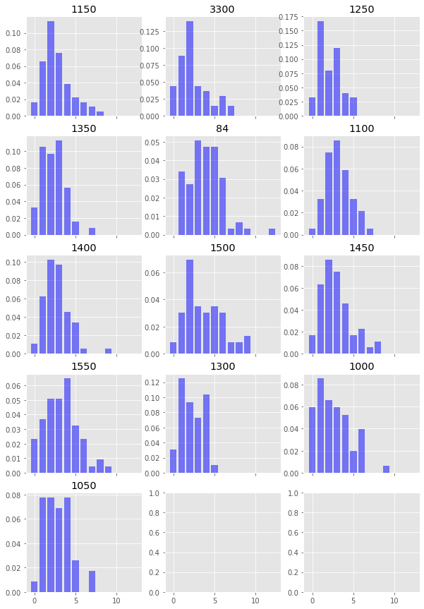
First, let’s plot the distribution of tries per team per game
import scipy.stats as stats


tries_per_game = df.groupby(['fxid', 'team_id']).max()['try_for']
fig, axes = plt.subplots(figsize=(10,15),nrows=5, ncols=3, sharex=True)

axes = axes.flatten()
for i,team in enumerate(tries_per_game.index.get_level_values(1).unique()):
    axes[i].set_title(team)
    axes[i].bar(
        tries_per_game.loc[:,team].value_counts().index,
        tries_per_game.loc[:,team].value_counts()/tries_per_game.loc[:,team].sum(),
        color='blue', alpha=0.5
    )
# Next let's calculate some parameters
mean = df.groupby(['fxid', 'team_id']).max()['try_for'].mean()
var = df.groupby(['fxid', 'team_id']).max()['try_for'].var()
p = mean / var
n = mean**2 / (var - mean)
# Create some samples from a negative binomial distribution
samples = stats.nbinom.rvs(n,p,size=10000)
sample_x, sample_y = np.unique(samples,return_counts=True)
Finally, let’s plot what our true try scoring distribution looks like (the blue bars) and overlay what our negative binomial distribution looks like (the red line).
import scipy.stats as stats


tries_per_game = df.groupby(['fxid', 'team_id']).max()['try_for']
fig, axes = plt.subplots(figsize=(10,15),nrows=5, ncols=3, sharex=True)

axes = axes.flatten()
for i,team in enumerate(tries_per_game.index.get_level_values(1).unique()):
    axes[i].set_title(team)
    axes[i].bar(
        tries_per_game.loc[:,team].value_counts().index,
        tries_per_game.loc[:,team].value_counts()/tries_per_game.loc[:,team].sum(),
        color='blue', alpha=0.5
    )

    ax2 = axes[i].twinx()
    ax2.set_yticks([])
    ax2.grid(False)
    ax2.plot(sample_x, sample_y/sample_y.sum())
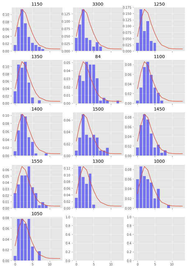
Conclusion
And there we have it, we can see that try scoring in Premiership rugby can be fairly accurately modelled by a negative binomial distribution and not a Poisson distibution which is used quite often in football.
Stay tuned for next week when I’ll be starting a mini series on recommendations combining graphs and image recognition…