Last week we built a Prog Rock knowledge graph using data from Wikidata and MusicBrainz. This week we’ll see how we can use Neo4j, Cypher and some of Neo4j’s Graph Data Science Library to create some insight from the knowledge graph. And as a bonus for coming back and reading this after part one, I’ll spare readers the tenuously linked Prog Rock related subheadings…
Which country produced the most Prog Rock bands?
As an introduction to Cypher’s aggregate functions, we’ll see which country out of UK and Italy produced the most bands. Unfortunately, when I originally created the knowledge graph, I filtered based on the bands formed in either the UK or Italy but I didn’t save this to the graph. So the first step was to query Wikidata to import this into the graph:
MATCH (b:Band)
WITH 'PREFIX sch: <http://schema.org/>
PREFIX rdfs: <http://www.w3.org/2000/01/rdf-schema#>
PREFIX wdt: <http://www.wikidata.org/prop/direct/>
PREFIX wd: <http://www.wikidata.org/entity/>
PREFIX rdf: <http://www.w3.org/1999/02/22-rdf-syntax-ns#>
CONSTRUCT {
  ?band a sch:Band ;
sch:countryOfOrigin ?country .
?country rdfs:label ?countryName .
 }
 WHERE {
     ?band wdt:P136 wd:Q49451. filter(?band = <' + b.uri +'> ).
     ?band wdt:P495 ?country ;
      rdfs:label ?bandName . filter (lang(?bandName) = "en") .
     ?country rdfs:label ?countryName. filter(lang(?countryName)  = "en") .
     SERVICE wikibase:label { bd:serviceParam wikibase:language "[AUTO_LANGUAGE]". }}'
     AS sparql, b
     CALL n10s.rdf.import.fetch(
         'https://query.wikidata.org/sparql?query=' + apoc.text.urlencode(sparql),
         "JSON-LD",
         { headerParams: { Accept: "application/ld+json"}, handleVocabUris:"MAP" }
     )
YIELD terminationStatus, triplesLoaded
RETURN b.name, terminationStatus, triplesLoaded
I then needed to relabel the countries because n10s automatically gives these nodes the label Resource (I assume there’s probably a better way to fetch the data from Wikidata via n10s to prevent this but I’ll go through the steps I ended up taking anyway).
MATCH ()-[r:countryOfOrigin]->(c)
SET c:Country
REMOVE c:Resource
Finally, add a name tag to each of the countries
MATCH ()-[r:countryOfOrigin]->(c)
SET c.name = CASE
WHEN c.uri CONTAINS 'Q21' THEN 'England'
WHEN c.uri CONTAINS 'Q38' THEN 'Italy'
ELSE 'United Kingdon' END
We can now run a simple query to count the number of bands from each country. You’ll notice that Cypher doesn’t need a GROUP BY function like a traditional SQL query, it automatically groups by any non-aggregated variables.
MATCH (c:Country)<-[o:countryOfOrigin]-() RETURN c.name, COUNT(o)
             ;
+-----------------------------+
| c.name           | COUNT(o) |
+-----------------------------+
| "United Kingdon" | 114      |
| "Italy"          | 36       |
| "England"        | 1        |
+-----------------------------+
And there we have it, 114 bands from the UK (115 technically as one was classed as England) and 36 from Italy.
Which bands have had the most members?
Another relatively simple one to familiarize ourselves with aggregation functions.
MATCH (m:Musician)-[rel:MEMBER_OF]->(b:Band)
RETURN b.name as bandName, COUNT(m) as countOfMembers
ORDER BY countOfMembers DESC LIMIT 5;
+---------------------------------+
| bandName       | countOfMembers |
+---------------------------------+
| "Uriah Heep"   | 23             |
| "Jethro Tull"  | 19             |
| "Renaissance"  | 19             |
| "King Crimson" | 18             |
| "Hawkwind"     | 17             |
+---------------------------------+
And we see that Uriah Heep are the merry-go round of the Prog Rock world. Whether they’re really a Prog Rock band could be up for debate but they did have multiple Roger Dean album covers so that probably qualifies them.
Which band has released the most music?
Let’s have a look at which band has released the most music by the total duration of all their tracks combined.
MATCH (t:Track)<-[:HAS_TRACK]-(a:Album)-[:RELEASED_BY]->(b:Band)
RETURN b.name as bandName, SUM(t.length)/60/1000/60 as totalLength
ORDER BY totalLength DESC LIMIT 5
╒══════════════╤═════════════╕
│"bandName"    │"totalLength"│
╞══════════════╪═════════════╡
│"Deep Purple" │101          │
├──────────────┼─────────────┤
│"Yes"         │93           │
├──────────────┼─────────────┤
│"Marillion"   │92           │
├──────────────┼─────────────┤
│"King Crimson"│90           │
├──────────────┼─────────────┤
│"Pink Floyd"  │88           │
└──────────────┴─────────────┘
In total, Deep Purple have released 101 hours of music including live albums, almost 8 hours more than the second placed band Yes.
6 Degrees of Progressive Separation
Let’s have a look at how the various band members are related based on whether they played together in a band. To start with, we need to create the relationship PLAYED_WITH between any pairs of musicians who were in the same band at some point (note that this doesn’t take into account which years each member was in a band as this data wasn’t readily available through Wikidata or MusicBrainz).
MATCH (m1:Musician)-[:MEMBER_OF]->(b:Band)<-[:MEMBER_OF]-(m2:Musician)
WHERE ID(m1) < ID(m2)
MERGE (m1)-[:PLAYED_WITH]->(m2)
We use the condition WHERE ID(m1) < ID(m2) so that we don’t create the relationship in both directions.
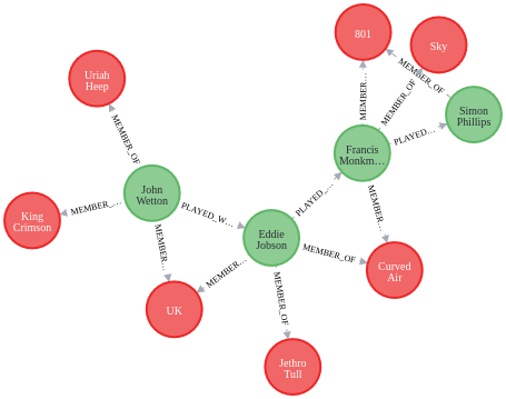
From here, we can start with a simple example of trying to find a path from King Crimson bassist John Wetton to drumming legend Simon Phillips using the shortestPath function.
MATCH (john:Musician {name: 'John Wetton'}), (simon:Musician {name: 'Simon Phillips'}),
p = shortestPath((john)-[a:PLAYED_WITH*]-(simon))
WITH p, nodes(p) as musicians
UNWIND musicians as musician
MATCH (musician)-[:MEMBER_OF]->(b:Band)
RETURN p, b
The results allow us to visualise the path from Wetton to Phillips via the various bands they’ve played in.
How well connected were the members of Asia?
For those who don’t already know, Asia were a Prog Rock super group formed in 1981 featuring members of King Crimson, Yes, The Bugles and ELP. Steve Carell even framed a poster of their debut album in the 40 Year Old Virgin

MATCH (m:Musician) WHERE
m.name = 'John Wetton' or
m.name = 'Carl Palmer' or
m.name = 'Geoff Downes' or
m.name = 'Steve Howe'
WITH collect(id(m)) AS asia
MATCH (m:Musician) WHERE NOT id(m) IN asia
WITH asia, collect(id(m)) as others
UNWIND asia AS a
UNWIND others AS o
MATCH (m:Musician) WHERE id(m) = a
MATCH (n:Musician) WHERE id(n) = o
MATCH p=shortestPath((m)-[rel:PLAYED_WITH*]-(n))
WITH m.name as memberName, collect(size(relationships(p))) as relLengths
RETURN memberName, reduce(totalRelLengths = 0, n in relLengths | totalRelLengths + n) AS totalRels, size(relLengths) as numRels

+--------------------------------------+
| memberName     | totalRels | numRels |
+--------------------------------------+
| "John Wetton"  | 455       | 198     |
| "Carl Palmer"  | 704       | 198     |
| "Geoff Downes" | 557       | 198     |
| "Steve Howe"   | 557       | 198     |
+--------------------------------------+
In the above query, we’re collecting all the members of Asia in one list, all other Musicians in another and then iterating over each pair of an Asia member and non-Asia member to find the shortest path between them. From there we collect the size of each path and use the reduce function to sum them all up. From the results, we can see that John Wetton was the best connected member of Asia with the lowest number of relationships needed to reach the 198 other musicians.
Community Detection
Next up, we will use Neo4j’s Graph Data Science Library (GDS) to see if we can detect communities with the Prog Rock Knowledge graph using the Louvain method. First off we need to create the projected graph containing Musicians and the relationships we want to use in the algorithm.
call gds.graph.create(
    'communityGraph',
    'Musician',
    {
        PLAYED_WITH: {
            orientation: 'UNDIRECTED'
        }
    }
)
From there, we can stream the results from the function and write the communities and intermediate communities back to the knowledge graph
CALL gds.louvain.stream('communityGraph', {includeIntermediateCommunities:true})
YIELD nodeId, communityId, intermediateCommunityIds
WITH gds.util.asNode(nodeId) AS nodes, communityId, intermediateCommunityIds
MERGE (c:Community {communityId: communityId})
MERGE (nodes)-[:IN_COMMUNITY]-(c)
WITH nodes, intermediateCommunityIds, c
UNWIND intermediateCommunityIds as icid
MERGE (d:Community {communityId: icid})
MERGE (nodes)-[:IN_INTERMEDIATE_COMMUNITY]-(d)
And now we can take some sample from the communities and see what patterns have emerged
MATCH p=(c:Community {communityId: 262})<-[com]-(m:Musician)-[member:MEMBER_OF]->(b:Band) RETURN p
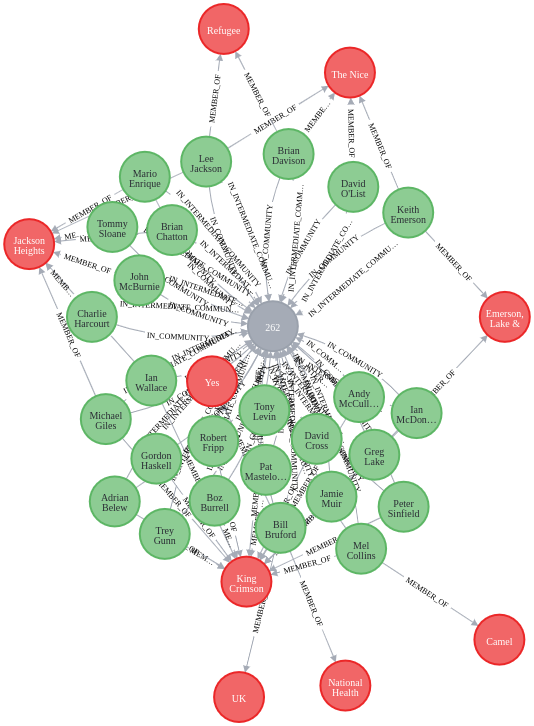
We can see that community 262 contains the founders of the English Prog rock scene in Yes, King Crimson and ELP.
MATCH p=(c:Community {communityId: 84})<-[com]-(m:Musician)-[member:MEMBER_OF]->(b:Band) RETURN p
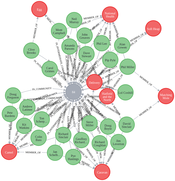
Community 84 contains many of the bands who started the Canterbury Prog Rock scene.
MATCH p=(c:Community {communityId: 153})<-[com]-(m:Musician)-[member:MEMBER_OF]->(b:Band) RETURN p
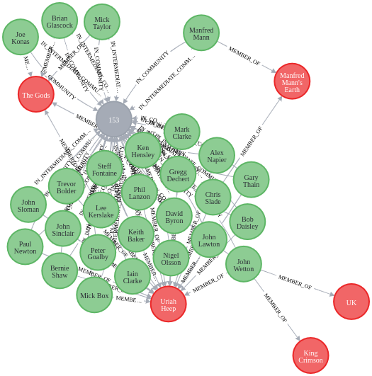
Finally, Community 153 seems to be defined by members and bands related to Uriah Heep.
Graph Embeddings
The last thing we’ll look at is using graph embeddings to represent the knowledge graph. This was done in Python using the Neo4j Python Connector.
Firstly, we need to create the embeddings using the FastRP algorithm. I’ve chosen 4 dimensions for the embeddings but in reality this could be larger in order to maintain as much info from the graph as possible.
query = """
CALL gds.fastRP.stream('musicians',
  {
    embeddingDimension: 4,
    randomSeed: 42
  }
)
YIELD nodeId, embedding
WITH gds.util.asNode(nodeId) as name, embedding
MATCH (name)-[:MEMBER_OF]->(b:Band)-[:COUNTRY_OF_ORIGIN]->(country:Country)
MATCH (name)-[:IN_COMMUNITY]->(c:Community)
RETURN name.name as musicianName, collect(DISTINCT b.name) as bandNames,
collect(DISTINCT country.name) as countries, collect(DISTINCT c.communityId) as community,
embedding
"""

with driver.session() as session:
    result = list(session.run(query))
This data can then be transferred into a Pandas DataFrame.
def create_df(results):
    data = {
        'musicians': [],
        'bands': [],
        'communities': [],
        'country': [],
        'embeddings0': [],
        'embeddings1': [],
        'embeddings2': [],
        'embeddings3': []
    }

    for row in results:
        data['musicians'].append(row['musicianName'])
        data['bands'].append(row['bandNames'])
        data['communities'].append(row['community'][0])
        data['country'].append(row['countries'][0])
        data['embeddings0'].append(row['embedding'][0])
        data['embeddings1'].append(row['embedding'][1])
        data['embeddings2'].append(row['embedding'][2])
        data['embeddings3'].append(row['embedding'][3])

    df = pd.DataFrame(data)

    return df

df = create_df(result)
I did experiment with plotting the embeddings as they were, but it was difficult to extract much info from the visualisation. Instead I looked at reducing the dimensionality of the dataset from 4 to 2 using PCA before plotting the embedding graph.
import numpy as np
from sklearn.decomposition import PCA

pca = PCA()
dft = pca.fit_transform(df[['embeddings0', 'embeddings1', 'embeddings2', 'embeddings3']])

pca.explained_variance_ratio_
>>> array([0.37460532, 0.24841197, 0.22309347, 0.15388925])
We can see from the last line that by using PCA, we can extract roughly 61% of the information from the data by using only 2 variables. We can now visualise how these embeddings transform the knowledge graph into traditional vectors. First we’ll take a few bands as examples for the visualisation.
kc_id = df[df['bands'].map(lambda x: 'King Crimson' in x)].index.values
yes_id = df[df['bands'].map(lambda x: 'Yes' in x)].index.values
pfm_id = df[df['bands'].map(lambda x: 'Premiata Forneria Marconi' in x)].index.values
heep_id = df[df['bands'].map(lambda x: 'Uriah Heep' in x)].index.values
other_id = [x for x in range(dft.shape[0]) if not x in np.r_[kc_id, yes_id, pfm_id]]
And then we can plot the data
plt.style.use('ggplot')
fig, ax = plt.subplots(figsize=(10,10))

ax.scatter(dft[other_id,0], dft[other_id,1], label='Others', s=50,alpha=.5, c='grey')
ax.scatter(dft[kc_id,0], dft[kc_id,1], label='King Crimson', s=200, c='r')
ax.scatter(dft[yes_id,0], dft[yes_id,1], label='Yes', s=200, c='b')
ax.scatter(dft[pfm_id,0], dft[pfm_id,1], label='PFM', s=200, c='g')
ax.scatter(dft[heep_id,0], dft[heep_id,1], label='Uriah Heep', s=200, c='brown')

ax.scatter(dft[52,0], dft[52,1], label='Bruford', s=200,alpha=1, c='purple')
ax.scatter(dft[115,0], dft[115,1], label='Wetton', s=200,alpha=1)

ax.legend()
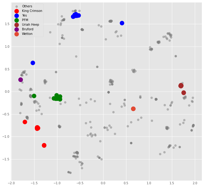
Interesting things we can see from the embeddings:
- Musicians from the same bands tend to be clustered together
- A musician who played in 2 different bands seems to sit halfway between each band. The two examples are Bill Bruford, who played in both Yes and King Crimson, and John Wetton who played in both King Crimson and Uriah Heep (both plotted individually on the graph). We can see that Bruford occupies a space in between the two bands he played in the same way that Wetton sits in between Crimson and Heep.
Closing Remarks
Overall I enjoyed building the knowledge graph and running some queries on it. I think there’s loads more I could so with the community detection algorithms and the embeddings but these were a good starting place to familiarise myself with the Neo4j tools and GDS library. If there are any questions or feedback then I’d love to hear it so please feel free to get in touch.