
Hi and welcome to another post continuing to look at dbt and its applications. The last post looked at using dbt to transform an open NCAA dataset in BigQuery and this week we’ll go a little further and look at some pro rugby data.
Background
One thing I’ve had chance to reflect on since leaving working in pro rugby is the various processes that need to occur to create robust, reusable and scalable analytics systems that can deliver up-to-date data quickly to the people who need/want it. Excel sheets on a shared Google Drive don’t really lend themselves to this process…just because they can be a solution, doesn’t mean they should.
So the purpose of this post is to look at how we can set up scalable, reusable and version controlled analytics code with the goal being to free up an analysts time from repetitive tasks and therefore be able to spend more time creating insight from the available data. We’ll look at this in s few different stages:
- Setting up the dbt project.
- Creating the various schemata to separate out the different parts of our project.
- Creating reusable code to deliver data to the analysts in a useful format.
Setting up the dbt Project
In terms of setting up the dbt project, it was a fairly standard setup i.e. creating a dbt project, linking to a BigQuery dataset and ensuring the various roles and permissions were in place and finally creating a GitHub repository.
The next step was to modify our dbt_project.yml to set the various parameters for our project. In terms of our models this looked as follows:
models:
  opta_stats:
    # Applies to all files under models/example/
    +materialized: view
    staging:
      +schema: staging
    marts:
      +matrialized: table
      core:
        +schema: core
      positional:
        +schema: positional
      intermediate:
        +schema: intermediate
We’ll first of all set out our default materialisation as view and then set out the hierarchy of folders and schemata. From here we also set the materialisation of any models under the marts directory to tables. The reason for this is to deliver the data as quick as possible when it’s needed. Views are quick to build but can be slow to query. Tables on the other hand are the opposite: slow to build but quicker to query. As the data grows, an analyst doesn’t want to be waiting every time they want to query the data from one of the marts tables. If we run our dbt models at a given interval, we can ensure the data is up to date and ready to be queried and that any time that would have been spent waiting for a complex view to query the dataset is saved by running the models at a separate time.
In terms of the project layout, my thinking was that we’ll need a staging layer (as always) to refer to each of the source tables. In dbt world, these should be the only models that refer to the source tables; all other tables to should refer to the staging tables. Next up we’ll need our marts layer where the data will be in a format ready to be used. We then further breakdown our marts layer into a core schema, a positional schema and an intermediate schema.
- The
intermediateschema - this contains (unsurprisingly) intermediate transformations of the data to be used in models further downstream. It’s in themartsfolder as these tables could also provide analysis in their own right but with the priority being to facilitate further transformations and analyses. - The
positionalschema - this layer of analysis would be position specific tables providing a bespoke analysis for each positional group. - The
coreschema - this would contain a generic level of analysis across all teams and players.
Diving in Deeper
I’ll not go into many of the staging models in detail as they’re all fairly similar and apply only the lightest transformations to the raw data (e.g. columns names changes and other soft transformations) but as an example here is one staging model:
with match_data as (

    select * from {{ source('opta_stats', 'match_data') }}

)

select * from match_data
Next, we’ll look at transforming some data to create an intermediate model to feed a position specific piece of analysis. Let’s assume we want to compare scrum halves box kicking abilities. We can first create an intermediate model that returns only the box kicks and some derived outcomes and then further process this to return our analysis.
We’ll start with the code for the intermediate model:
with box_kicks as (

    select
        match_data.plid as plid,
        match_data.fxid as fxid,
        match_data.actiontype as action_type,
        descriptions.qualifier_descriptor as action_result,
        case
          when y_coord_end <= 15 or y_coord_end >=55 then true
          else false end
        as landed_in_fifteens

    from {{ ref('stg_match_data') }} as match_data
    inner join {{ ref('stg_descriptions') }} as descriptions
    on match_data.actionresult = descriptions.qualifier

    where match_data.actiontype = 346

)

select * from box_kicks
A fairly simple model - we get each instance of a box quick and transform the outcome so we have a simple indicator as to whether the kick landed in the 15m channel (yes, this will depend on the context and situation of the kick but in general this is the target).
We can then use this is our position specific model:
{% set outcomes = dbt_utils.get_column_values(table=ref('intermediate__scrum_half'), column='action_result') %}

with kick_totals as (

    select
        plid,
        count(distinct fxid) as num_game,
        count(1) as num_kicks,
        round(count(case when landed_in_fifteens is true then 1 else null end) / count(1) * 100, 1) as landed_in_15_rate,

        {% for outcome in outcomes %}
            {% set outcome_label = modules.re.sub('[ \-()]', '_', outcome) | lower %}
                round(count(case when action_result = '{{ outcome }}' then 1 else null end) / count(1) * 100, 1) as {{ outcome_label }} {% if not loop.last %},{% endif %}
        {% endfor %}


    from {{ ref('intermediate__scrum_half') }}

    group by 1

),

player_minutes as (

    select
        plid,
        sum(mins) as mins_played

    from {{ ref('stg_team_data') }} as team_data

    where exists (

        select 1
        from {{ ref('stg_team_data') }} as team_data_b
        where team_data.plid = team_data_b.plid
        and team_data_b.posid = 9
    )

    group by 1

),

kicks_per_min as (

    select
        players.plforn || ' ' || players.plsurn as player_name,
        player_minutes.mins_played as mins_played,
        round(kick_totals.num_kicks / player_minutes.mins_played * 80, 2) as kicks_per_80,
        kick_totals.*

from kick_totals
inner join player_minutes using (plid)
inner join {{ ref('stg_players') }} as players using (plid)

)

select * from kicks_per_min
Let’s break this down piece by piece…
{% set outcomes = dbt_utils.get_column_values(table=ref('intermediate__scrum_half'), column='action_result') %}
In the first part we’re using a dbt_utils function to get the unique values in a column from another model. This is the equivalent of select distinct action_type from table and returning the values as a list. We’ll go on to use this when we pivot the data.
with kick_totals as (

    select
        plid,
        count(distinct fxid) as num_game,
        count(1) as num_kicks,
        round(count(case when landed_in_fifteens is true then 1 else null end) / count(1) * 100, 1) as landed_in_15_rate,

        {% for outcome in outcomes %}
            {% set outcome_label = modules.re.sub('[ \-()]', '_', outcome) | lower %}
                round(count(case when action_result = '{{ outcome }}' then 1 else null end) / count(1) * 100, 1) as {{ outcome_label }} {% if not loop.last %},{% endif %}
        {% endfor %}


    from {{ ref('intermediate__scrum_half') }}

    group by 1

)
The purpose of this snippet is find each player, the number of games they’ve played in and the rate of which the box kicks landed in a 15m channel. We also use the outcome of our get_column_values function to pivot the table by iterating though the list and creating a column for each outcome. One thing we have to do though is use a modules.re.sub('[ \-()]', '_', outcome) to ensure the label can also be used as a column name i.e, it contains no spaces or hyphens.
Next we need to filter this down to only those players who have ever played scrum half and calculate the number of minutes they have played:
player_minutes as (

    select
        plid,
        sum(mins) as mins_played

    from {{ ref('stg_team_data') }} as team_data

    where exists (

        select 1
        from {{ ref('stg_team_data') }} as team_data_b
        where team_data.plid = team_data_b.plid
        and team_data_b.posid = 9
    )

    group by 1

)
Another fairly simple CTE where we reference the team sheet data from all the matches to find only those who have ever played at 9 and then sum up the minutes played.
Finally we create the usable output:
kicks_per_min as (

    select
        players.plforn || ' ' || players.plsurn as player_name,
        player_minutes.mins_played as mins_played,
        round(kick_totals.num_kicks / player_minutes.mins_played * 80, 2) as kicks_per_80,
        kick_totals.*

from kick_totals
inner join player_minutes using (plid)
inner join {{ ref('stg_players') }} as players using (plid)

)

select * from kicks_per_min
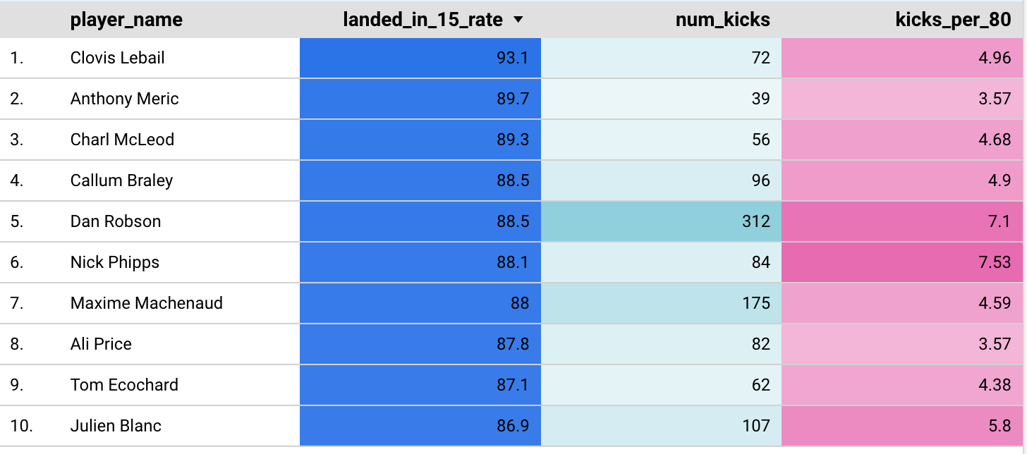
And now once we’ve run this query let’s have a look at the output - we’ll get the scrum halves with the highest percentage of kicks that landed in a 15m channel given that they’ve played the equivalent of at least 10 full games
select * from {{ ref('scrum_half_box_kick') }}
where mins_played >= 800
and kicks_per_80 > 3
order by landed_in_15_rate desc
So there we have it…a reusable, scalable and traceable analytics model which can be updated regularly. All we need to do is ensure we keep the source data up to date.
I’ll spare all the code of another example (you can find it on the GitHub repo), but here’s a subset of the results for our back row model, ordered by jackal_success_odds i.e. the odds ratio of successful to unsuccessful jackal attempts. A score of 1 represents an equal number of successful and failed attempts. A score of 5 would show 5 times as many successful attempts as unsuccessful attempts.
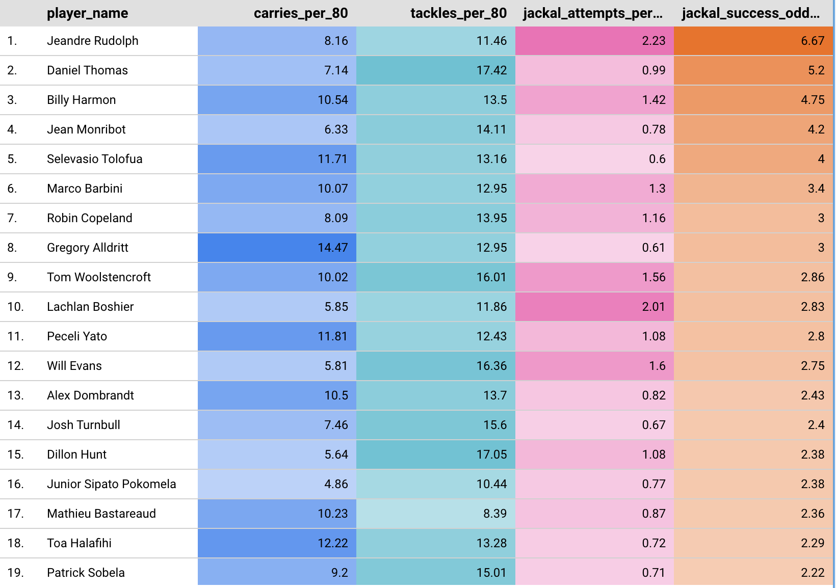
Note Mathieu Bastareaud presence in the back row analysis - apparently he has converted to a number 8 full time these days whilst playing in America. I’ll dive into some other metrics in next weeks post.