
I’ve recently been working through an excellent resource on causal inference from Matheus Facure. Machine learning models are great at predicting things (well, in some cases…*cough* Zillow *cough*). You throw some data at them, make some predictions and try to find a model which gives you the best accuracy (or whatever measure it is you’re trying to optimize). Some models may be explainable as to why they make their predictions and some are black box models which can be incredibly difficult to interpret which in turn runs the risk of a lack of trust in the predictions. However, consider a machine learning model trained on airline prices…it would see that ticket sales a relatively low when the prices are low (during term time for example) and ticket sales go up as prices go up (during school holidays). A naive model may suggest increasing prices to increase sales…

ML models aren’t so great at answering the ‘what if’ questions…“what would happen if I changed the price of X?”, “How do socio-economic factors affect Y?”. Although it’s relatively easy to spot association patterns in data, what we really want to examine are the causal patterns. How can we figure out when an association is actually a causation?
For a more in depth analysis, I’d suggest having a look at:
- Matheus Facure’s resource
- Mastering Metrics
In this post I’m going to explore the omitted variable bias - how biased are the parameters we estimate from our model and how are these affected by the inclusion and exclusion of selected variables.
Omitted Variable Bias
I’ll use a very simple example to work through this. Estimating points scored by a rugby team from number of tries, conversions and penalties. But wait, eagle eyed readers will realise this is completely deterministic so we’ll add some randomness to the data as if it were a stochastic process - let’s assume that depending on the amount or lack of ‘jouer’ involved in the build up to a try, the referee can award +/- a normally distributed variable with zero mean and a standard deviation of 5. What a world that would be to live in…
Anyway, the dataset is a couple seasons worth of match data containing the points scored, tries, conversions and penalty kicks. Our data should now meet the 4 assumptions associated with a linear regression model:
- Linearity: The relationship between X and the mean of Y is linear.
- Homoscedasticity: The variance of residual is the same for any value of X.
- Independence: Observations are independent of each other.
- Normality: For any fixed value of X, Y is normally distributed..
import pandas as pd
import numpy as np
import matplotlib.pyplot as plt
import statsmodels.formula.api as smf

df = pd.read_csv('rugby_regression.csv', index_col=0)
df.columns = ['tries', 'conversions', 'penalty_goals', 'points']
# Add some randomness to the data
df['points'] = df['points'] + np.random.normal(loc=0, scale=5, size=df.shape[0])
# Remove any scores below zero
df.loc[df['points'] < 0, 'points'] = 0
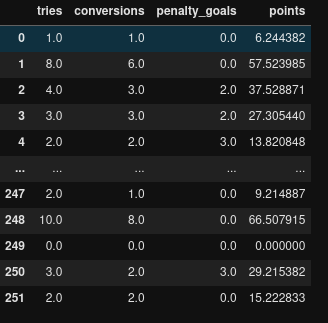
And we end up with a dataset looking something like this…
If we include all of these variables in our regression model (which will be known as the ‘long model’), this would be:
\[\hat {Points}_i = \beta_0 + \beta_1 \cdot {Tries}_i + \beta_2 \cdot {Conversions}_i + \beta_3 \cdot {Penalty Goals}_i + u_i\]That is, our predicted points are a linear combination of tries, conversions and penalties plus our error term, $u$. Now if we run a linear regression of points on tries, conversions and penalties, it should be fairly easy to figure out what each of the coefficients will be…

If you said 5, 2 and 3 then give yourself a pat on the back. So let’s double check this:
long_model = smf.ols('points ~ tries + conversions + penalty_goals', data=df).fit()
long_model.summary()

=================================================================================
                    coef    std err          t      P>|t|      [0.025      0.975]
---------------------------------------------------------------------------------
Intercept        -0.4382      0.872     -0.503      0.616      -2.155       1.279
tries             4.9084      0.357     13.767      0.000       4.206       5.611
conversions       2.1994      0.398      5.525      0.000       1.415       2.983
penalty_goals     3.2257      0.261     12.375      0.000       2.712       3.739
=================================================================================
Our model has estimated these parameters fairly well. If we hadn’t added our ref’s try bonus to our data then these values would be exactly 5, 2 and 3 as expected.
The Short Model
So now imagine we’re in a situation whereby we only have the number of tries available to us but we want to estimate the number of points scored by each team, in this case our model looks more like (where $u_i$ is the error term):
\[\hat {Points}_i = \beta_0 + \beta_1 \cdot {Tries}_i + u_i\]What happens if we run this regression now?
really_short_model = smf.ols('points ~ tries', data=df).fit()
print(really_short_model.summary().tables[1])

==============================================================================
                 coef    std err          t      P>|t|      [0.025      0.975]
------------------------------------------------------------------------------
Intercept      6.5686      0.890      7.383      0.000       4.816       8.321
tries          5.6777      0.239     23.792      0.000       5.208       6.148
==============================================================================
If we don’t include anything other than the number of tries scored in our model, the best fit for the model estimates a baseline score of 6,57 and that a try is worth 5.7 points +/- ~0.5. We now have a biased estimator - essentially the coefficient of the tries variable is trying to account for the other missing variables.
Another way of estimating this coefficient is:
\(\beta_1^{*} = \frac{Cov(Y_i, x_{1i})}{Var(x_{1i})}\)
beta_1_biased = df['points'].cov(df['tries']) / df['tries'].var()
print(beta_1_biased)

>>> 5.677674982234511
The age old saying goes something like this:
“Short equals long plus the effect of omitted times the regression of omitted on included”
Which means the parameters from our short model should be equal to the coefficients for our long model + the effect of omitted variable in the long model multiplied by the regression of each omitted variable on the included variable.
We can see what this looks like in when we calculate it to make sense of it. $\beta_1$ can be calculated as follows: \(\beta_1^{*} = \beta_1 + \beta_2 \delta_{21} + \beta_3 \delta_{31}\)
where
\[\delta_{21} = \frac{Cov(X_{2i}, X_{1i})}{Var(X_{1i})}\] \[\delta_{31} = \frac{Cov(X_{3i}, X_{1i})}{Var(X_{1i})}\]The $\delta$ values are calculated by running a regression of the included variable (in this case, tries scored) on each of the excluded variables to account for the contribution of each of these variables to the coefficient for the variable included in our model.
# From our long model
beta_1 = 4.91
beta_2 = 2.20
beta_3 = 3.22

# regression of omitted on included variables
delta_1 = df['conversions'].cov(df['tries']) / df['tries'].var()
delta_2 = df['penalty_goals'].cov(df['tries']) / df['tries'].var()

# Proving short equals long 'mantra'
beta_1_biased = beta_1 + beta_2*delta_1 + beta_3*delta_2

print(beta_1_biased)

# Close enough - rouding errors!
>>> 5.681167904903418
Positive or Negative bias?
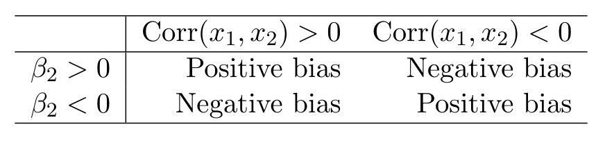
And given we can safely assume that the number of tries is positively correlated with the number of conversions and that our coefficient is positive, we can see that we have a positive bias in our parameters.
Using Multiple Variables
I could find lots of examples online of including only one variable in the short model and excluding the rest, but it was a bit more difficult to find a good example where we include multiple variables…now there is the complication of removing the influence of each of the included variables on each other.

So let’s look at another example and in this case we’ll look at a model that includes both tries and conversions but excludes penalties.
short_model = smf.ols('points ~ tries + conversions', data=df).fit()
print(short_model.summary().tables[1])

===============================================================================
                  coef    std err          t      P>|t|      [0.025      0.975]
-------------------------------------------------------------------------------
Intercept       6.6378      0.835      7.946      0.000       4.993       8.283
tries           3.5198      0.430      8.194      0.000       2.674       4.366
conversions     2.9410      0.499      5.888      0.000       1.957       3.925
===============================================================================
Now we have a model which estimates a baseline score of 6.6, tries are worth ~3.5 points and conversions worth 2.9. Clearly we have a biased model due to the omission of the penalty variable.
Now when looking at our coefficients, we need to remove the influence of the included variables on each other when accounting for our biased parameters.
If we include two variables (tries and conversions) and exclude one (penalties), then $\beta_1$ (the coefficient for tries scored) should be:
\[\beta_1^{*} = \beta_1 + \beta_3 \delta_{31}\]where
\[\delta_{31} = \frac{Cov(X_{3i}, \tilde x_{1i})}{Var(\tilde x_{1i})}\]and $\tilde x_{1i}$ is the residuals of the regression of $X_1$ (tries scored) on the remaining included variables (conversions).
We can see what’s happening when we code this out…
# Regression of our variable of interest on the other included variables
tries_on_coversions = smf.ols('tries ~ conversions', data=df).fit()

# Use our model to predict tries from conversions
predictions = tries_on_coversions.predict(df['conversions'])

# Calculate the residuals (delta in our model)
residuals = df['tries'] - predictions

# Regression of the omitted variables on the residual of the included
reg_omitted_included = df['penalty_goals'].cov(residuals) / residuals.var()
print(beta_1 + beta_3 * reg_omitted_included)

>>> 3.5237958437354404
And similarly if we look at the coefficient for conversions:
# Regression of our variable of interest on the other included variables
conversions_on_tries = smf.ols('conversions ~ tries', data=df).fit()

# Use our model to predict tries from conversions
predictions = conversions_on_tries.predict(df['tries'])

# Calculate the reisduals (delta in our model)
residuals = df['conversions'] - predictions

# Regression of the omitted variables on the residual of the included
reg_omitted_included = df['penalty_goals'].cov(residuals) / residuals.var()

print(beta_2 + beta_3 * reg_omitted_included)
>>> 2.940282294787459
Closing Remarks
This concludes my rambling about the omitted variable bias. Although the dataset was somewhat artificial, hopefully it’s been a useful exercise for looking how the inclusion or exclusion of certain variables can affect the parameters of our model. I’d highly recommend the resources I linked to at the start of the post for a much better explanation of causal inference.